FIN435 Class Web
Page, Spring '24
Jacksonville
University
Instructor:
Maggie Foley
The Syllabus Overall Grade calculator
Exit Exam Questions (will be posted in week 10 on blackboard)
Term Project (on efficient
frontier, updated, due with final)
Weekly SCHEDULE, LINKS, FILES and Questions
|
Week |
Coverage, HW, Supplements -
Required |
|
Reading Materials |
||||||||||||||||||||||||||||||||||||||||||||||||||||||||||||||||||||||||||||||||||||||||||||||||||||||||||||||||||||||||||||||||||||||||||||||||||||||||||||||||||||||||||||||||||||||||||||||||||||||||||||||||||||||||||||||||||||||||||||||||||||||||||||||||||||||||||||||||||||||||||||||||||||||||||||||||||||||||||||||||||||||||||||||||||||||||||||||||||||||||||||||||||||||||||||||||||||||||||||||||||||||||||||||||||||||||||||||||||||||||||||||||||||||||||||||||||||||||||||||||||||||||||||||||||||||||||||||||||||||||||||||||||||||||||||||||||||||||||||||||||||||||||||||||||||||||||||||||||||||||||||||||||||||||||||||||||||||||||||||||||||||||||||||||||||||||||||||||||||||||||||||||||||||||||||||||||||||||||||||||||||||||||||||||||||||||||||||||||||||||||||||||||||||||||||||||||||||||||||||||||||||||||||||||||||||||||||||||||||||||||||||||||||||||||||||||||||||||||||||||||||||||||||||||||||||||||||||||||||||||||||||||||||||||||||||||||||||||||||||||||||||||||||||||||||||||||||||||||||
|
Week 1 |
Marketwatch Stock Trading Game (Pass code: havefun) Risk Tolerance Test https://jufinance.com/risk_tolerance.html
1. URL for your game: 2. Password for this private game: havefun. 3. Click on the 'Join Now' button to get
started. 4. If you are an existing MarketWatch member, login. If you are a new user,
follow the link for a Free account - it's easy! 5. Follow the instructions and start trading! 6. Game will be over
on 4/22/2022 How to Use Finviz Stock
Screener (youtube, FYI)
How To Win The MarketWatch Stock
Market Game (youtube, FYI)
How Short Selling Works (Short
Selling for Beginners) (youtube, FYI)
|
|
|
||||||||||||||||||||||||||||||||||||||||||||||||||||||||||||||||||||||||||||||||||||||||||||||||||||||||||||||||||||||||||||||||||||||||||||||||||||||||||||||||||||||||||||||||||||||||||||||||||||||||||||||||||||||||||||||||||||||||||||||||||||||||||||||||||||||||||||||||||||||||||||||||||||||||||||||||||||||||||||||||||||||||||||||||||||||||||||||||||||||||||||||||||||||||||||||||||||||||||||||||||||||||||||||||||||||||||||||||||||||||||||||||||||||||||||||||||||||||||||||||||||||||||||||||||||||||||||||||||||||||||||||||||||||||||||||||||||||||||||||||||||||||||||||||||||||||||||||||||||||||||||||||||||||||||||||||||||||||||||||||||||||||||||||||||||||||||||||||||||||||||||||||||||||||||||||||||||||||||||||||||||||||||||||||||||||||||||||||||||||||||||||||||||||||||||||||||||||||||||||||||||||||||||||||||||||||||||||||||||||||||||||||||||||||||||||||||||||||||||||||||||||||||||||||||||||||||||||||||||||||||||||||||||||||||||||||||||||||||||||||||||||||||||||||||||||||||||||||||||
|
Chapter 6 Interest rate Chapter summary 1) Shape of Yield Curve i) Inverted Yield Curve Indicates Recession:
The shape of the yield curve, particularly when inverted, serves as a
significant indicator of an impending recession. 2) Expectation Theory 3) Interest Rate Breakdown i) Breaking down interest rates involves
considering various components: Real Interest
Rate Inflation
Premium: Default
Premium: Liquidity
Premium:
Maturity Premium: For
class discussion: Interest Rate Volatility: ·
What factors could explain the recent
spike in interest rates compared to a year ago? Economic Conditions and
Rates: ·
How do economic indicators like inflation,
unemployment, and GDP growth contribute to the determination of interest
rates? Central Banks' Role: ·
What role do central banks play in setting
and adjusting interest rates, and how does their decision-making impact the
economy? Global Economic Influence: ·
How do international economic conditions
and events contribute to fluctuations in domestic interest rates? Impact on Borrowers and
Savers: ·
Discuss the effects of high interest rates
on borrowers and savers, both at the individual and business levels. Investor Behavior: ·
How does investor behavior respond to
changes in interest rates, and what role does sentiment play in influencing
rate movements? Part I: Who determines interest rates in the US? Market data website: Market watch on Wall Street Journal has daily yield curve and
interest rate information.
|
|||||||||||||||||||||||||||||||||||||||||||||||||||||||||||||||||||||||||||||||||||||||||||||||||||||||||||||||||||||||||||||||||||||||||||||||||||||||||||||||||||||||||||||||||||||||||||||||||||||||||||||||||||||||||||||||||||||||||||||||||||||||||||||||||||||||||||||||||||||||||||||||||||||||||||||||||||||||||||||||||||||||||||||||||||||||||||||||||||||||||||||||||||||||||||||||||||||||||||||||||||||||||||||||||||||||||||||||||||||||||||||||||||||||||||||||||||||||||||||||||||||||||||||||||||||||||||||||||||||||||||||||||||||||||||||||||||||||||||||||||||||||||||||||||||||||||||||||||||||||||||||||||||||||||||||||||||||||||||||||||||||||||||||||||||||||||||||||||||||||||||||||||||||||||||||||||||||||||||||||||||||||||||||||||||||||||||||||||||||||||||||||||||||||||||||||||||||||||||||||||||||||||||||||||||||||||||||||||||||||||||||||||||||||||||||||||||||||||||||||||||||||||||||||||||||||||||||||||||||||||||||||||||||||||||||||||||||||||||||||||||||||||||||||||||||||||||||||||||||||

|
Date |
1 Mo |
2 Mo |
3 Mo |
4 Mo |
6 Mo |
1 Yr |
2 Yr |
3 Yr |
5 Yr |
7 Yr |
10 Yr |
20 Yr |
30 Yr |
|
01/02/2024 |
5.55 |
5.54 |
5.46 |
5.41 |
5.24 |
4.80 |
4.33 |
4.09 |
3.93 |
3.95 |
3.95 |
4.25 |
4.08 |
|
01/03/2024 |
5.54 |
5.54 |
5.48 |
5.41 |
5.25 |
4.81 |
4.33 |
4.07 |
3.90 |
3.92 |
3.91 |
4.21 |
4.05 |
|
01/04/2024 |
5.56 |
5.48 |
5.48 |
5.41 |
5.25 |
4.85 |
4.38 |
4.14 |
3.97 |
3.99 |
3.99 |
4.30 |
4.13 |
|
01/05/2024 |
5.54 |
5.48 |
5.47 |
5.41 |
5.24 |
4.84 |
4.40 |
4.17 |
4.02 |
4.04 |
4.05 |
4.37 |
4.21 |
|
01/08/2024 |
5.54 |
5.48 |
5.49 |
5.39 |
5.24 |
4.82 |
4.36 |
4.11 |
3.97 |
3.99 |
4.01 |
4.33 |
4.17 |
|
01/09/2024 |
5.53 |
5.46 |
5.47 |
5.38 |
5.24 |
4.82 |
4.36 |
4.09 |
3.97 |
4.00 |
4.02 |
4.33 |
4.18 |
In class exercise – based on the above table,
·
Draw yield curve on 1/2/2024, and 1/9/2024.
·
Why do interest rates change on a daily basis?
1. What is the term structure
of interest rates based on the provided yield curve data?
A) Inverted
B) Flat
C) Normal
Answer: A
Explanation: An inverted yield curve often suggests
market expectations of economic downturn.
2. Which maturity shows the
highest interest rate in the data?
A) 1 month
B) 10 Years
C) 30 Years
Answer: A
Explanation: The yield for the 1-month maturity is
5.5%, the highest among the options.
3. What does a
downward-sloping yield curve suggest about market expectations?
A) Economic expansion
B) Economic contraction
C) Stable economic
conditions
Answer: B
Explanation: An inverted yield curve often indicates
expectations of economic downturn.
4. How does the yield for
the 10-year maturity compare to the 1-year maturity on 01/05/2024?
A) Higher
B) Lower
C) Equal
Answer: B
Explanation: The yield for the 10-year maturity
(4.05%) is lower than the 1-year maturity (4.84%).
5. Based on the data, what
can be inferred about market confidence in the short term?
A) High confidence
B) Low confidence
C) Stable confidence
Answer: B
Explanation: Short-term yields are relatively high,
indicating potential uncertainty or risk. Remember: Price and yield tend to
move in opposite direction.
6. If the yield for the
3-month maturity decreases significantly, what might this signal about
short-term economic expectations?
A) Economic expansion
B) Economic contraction
C) Stable economic
conditions
Answer: A
Explanation: A decrease in short-term yields could
suggest increased confidence in economic growth.
Treasury Inflation Protected Securities (TIPS)
|
NAME |
COUPON |
PRICE |
YIELD |
1 MONTH |
1 YEAR |
TIME (EST) |
|
GTII5:GOV 5 Year |
2.38 |
102.79 |
1.76% |
-32 |
+25 |
2:46 AM |
|
GTII10:GOV 10 Year |
1.38 |
96.48 |
1.78% |
-21 |
+40 |
2:46 AM |
|
GTII20:GOV 20 Year |
0.75 |
80.63 |
2.03% |
-8 |
+48 |
2:46 AM |
|
GTII30:GOV 30 Year |
1.50 |
89.28 |
1.99% |
-3 |
+51 |
2:46 AM |
https://www.bloomberg.com/markets/rates-bonds/government-bonds/us
·
Expected
Inflation=5-year Treasury yield rate − 5-year
TIPS rate
In this
formula, the 10-year Treasury yield rate is indeed expected to be higher than
the 10-year TIPS rate. The rationale is that the nominal Treasury yield
includes both the real interest rate and the market's expectation for
inflation, while the TIPS rate provides the real interest rate. Therefore,
subtracting the TIPS rate from the Treasury yield gives an estimate of the
market's expectation for inflation over the specified period.
In
Class Exercise:
·
What is TIPs?
Who Determines Interest Rates?
https://www.investopedia.com/ask/answers/who-determines-interest-rates/
By NICK K.
LIOUDIS Updated Aug 15, 2019
Interest rates are the cost
of borrowing money. They represent what creditors earn for lending you money.
These rates are constantly changing, and differ based on the lender, as well
as your creditworthiness. Interest rates not only keep the economy
functioning, but they also keep people borrowing, spending, and lending. But
most of us don't really stop to think about how they are implemented or who
determines them. This article summarizes the three main forces that control
and determine interest rates.
KEY TAKEAWAYS
- Interest rates are the cost of
borrowing money and represent what creditors earn for lending money.
- Central banks raise or lower
short-term interest rates to ensure stability and liquidity in the
economy.
- Long-term interest rates are affected
by demand for 10- and 30-year U.S. Treasury notes.
- Low demand for long-term notes leads
to higher rates, while higher demand leads to lower rates.
- Retail banks also control rates based on the market,
their business needs, and individual customers.
Short-Term Interest Rates: Central Banks
In countries using a centralized
banking model, short-term interest rates are determined by central banks. A
government's economic observers create a policy that helps ensure stable
prices and liquidity. This policy is routinely checked so the supply of money
within the economy is neither too large, which causes prices to increase, nor
too small, which can lead to a drop in prices.
In the U.S., interest rates
are determined by the Federal Open Market
Committee (FOMC), which consists
of seven governors of the Federal Reserve Board and five Federal Reserve Bank
presidents. The FOMC meets eight times a year to determine the near-term
direction of monetary policy and interest rates. The actions of central banks
like the Fed affect short-term and variable interest rates.
If the monetary policymakers
wish to decrease the money supply, they will raise the interest rate, making
it more attractive to deposit funds and reduce borrowing from the central
bank. Conversely, if the central bank wishes to increase the money supply,
they will decrease the interest rate, which makes it more attractive to
borrow and spend money.
The Fed funds rate affects the prime rate—the rate banks charge their
best customers, many of whom have the highest credit rating possible. It's
also the rate banks charge each other for overnight loans.
The U.S.
prime rate remained at 3.25% between Dec. 16, 2008 and Dec. 17, 2015, when it
was raised to 3.5%.
Long-Term
Interest Rates: Demand for Treasury Notes
Many of these rates are independent of the Fed funds rate,
and, instead, follow 10- or 30-year Treasury note yields. These yields depend on demand after the U.S. Treasury
Department auctions them off on the market. Lower demand tends to result in high interest rates. But when there
is a high demand for these notes, it can push rates down lower.
If you have a long-term
fixed-rate mortgage, car loan, student loan, or any similar non-revolving consumer
credit product, this is where it falls. Some credit card annual percentage
rates are also affected by these notes.
These rates are generally
lower than most revolving credit products but are higher than the prime rate.
Many savings account rates are also determined by long-term
Treasury notes.
Other
Rates: Retail Banks
Retail banks are also partly responsible for controlling interest
rates. Loans and mortgages they offer may
have rates that change based on several factors including their needs, the
market, and the individual consumer.
For example, someone with a
lower credit score may be at a higher risk of default, so they pay a higher
interest rate. The same applies to credit cards. Banks will offer different
rates to different customers, and will also increase the rate if there is a
missed payment, bounced payment, or for other services like balance transfers
and foreign exchange.
In class exercise:
1.
Who
is responsible for determining short-term interest rates in a centralized
banking model?
A) Commercial Banks
B) Central Banks
C) Government Agencies
Answer: B
Explanation: In countries with a centralized banking model,
short-term interest rates are determined by central banks.
2.
What
committee in the U.S. is responsible for setting interest rates and monetary
policy?
A) Federal Trade Commission
(FTC)
B) Federal Reserve Act
Committee (FRAC)
C) Federal Open Market Committee
(FOMC)
Answer: C
Explanation: The FOMC, consisting of governors of the
Federal Reserve Board and Federal Reserve Bank presidents, determines the
near-term direction of monetary policy and interest rates in the U.S.
3.
How
does a central bank decrease the money supply in the economy?
A) Increasing interest rates
B) Lowering interest rates
C) Printing more money
Answer: A
Explanation: Raising interest rates makes it more
attractive to deposit funds, reducing borrowing and decreasing the money
supply.
4.
Which
factor primarily influences the yields of 10- or 30-year Treasury notes?
A) Federal Reserve decisions
B) Market demand
C) Commercial bank policies
Answer: B
Explanation: The yields of Treasury notes depend on
demand in the market after auctions by the U.S. Treasury Department.
5.
What
happens to interest rates when there is high demand for Treasury notes?
A) Rates increase
B) Rates decrease
C) Rates remain unchanged
Answer: B
Explanation: High demand for Treasury notes tends to push
interest rates down.
6.
Who
determines interest rates on loans and mortgages offered by retail banks?
A) Government agencies
B) Central banks
C) Retail banks
Answer: C
Explanation: Retail banks control the interest rates
on the loans and mortgages they offer.
7.
Why might an individual with a lower credit
score be charged a higher interest rate?
A) Higher credit risk
B) Lower credit risk
C) Government regulations
Answer: A
Explanation: Individuals with lower credit scores are
considered higher risk, leading to higher interest rates.
Part II: Shapes of Yield Curve
For class
discussion: What
factors contributed to the shifts in yield curve shapes in 2023?

Data:
|
Date |
1 Mo |
2 Mo |
3 Mo |
6 Mo |
1 Yr |
2 Yr |
3 Yr |
5 Yr |
7 Yr |
10 Yr |
20 Yr |
30 Yr |
|
1/6/2020 |
1.54 |
1.54 |
1.56 |
1.56 |
1.54 |
1.54 |
1.56 |
1.61 |
1.72 |
1.81 |
2.13 |
2.28 |
|
1/6/2021 |
0.09 |
0.09 |
0.09 |
0.09 |
0.11 |
0.14 |
0.2 |
0.43 |
0.74 |
1.04 |
1.6 |
1.81 |
|
1/6/2022 |
0.04 |
0.05 |
0.1 |
0.23 |
0.45 |
0.88 |
1.15 |
1.47 |
1.66 |
1.73 |
2.12 |
2.09 |
|
1/6/2023 |
4.32 |
4.55 |
4.67 |
4.79 |
4.71 |
4.24 |
3.96 |
3.69 |
3.63 |
3.55 |
3.84 |
3.67 |
|
1/5/2024 |
5.54 |
5.48 |
5.47 |
5.24 |
4.84 |
4.4 |
4.17 |
4.02 |
4.04 |
4.05 |
4.37 |
4.21 |
Monday 1/15/2020
For daily yield curve, please visit https://www.gurufocus.com/yield_curve.php

Understanding the yield curve (video)
Introduction to the yield curve (khan academy)
Summary of Yield Curve Shapes and Explanations
Normal Yield Curve
When bond investors expect the economy to hum along at normal rates of growth
without significant changes in inflation rates or available capital, the
yield curve slopes gently upward. In the absence of economic disruptions,
investors who risk their money for longer periods expect to get a bigger
reward — in the form of higher interest — than those who risk their money for
shorter time periods. Thus, as maturities lengthen, interest rates get
progressively higher and the curve goes up.
Steep Curve –
Economy is improving
Typically the yield on 30-year Treasury bonds is three percentage points
above the yield on three-month Treasury bills. When it gets wider than that —
and the slope of the yield curve increases sharply — long-term bond holders
are sending a message that they think the economy will improve quickly in the
future.
Inverted Curve –
Recession is coming
At first glance an inverted yield curve seems like a paradox. Why would
long-term investors settle for lower yields while short-term investors take
so much less risk? The answer is that long-term investors will settle for
lower yields now if they think rates — and the economy — are going even lower
in the future. They're betting that this is their last chance to lock in
rates before the bottom falls out.

Flat
or Humped Curve
To become inverted, the yield curve
must pass through a period where long-term yields are the same as short-term
rates. When that happens the shape will appear to be flat or, more commonly,
a little raised in the middle.
Unfortunately, not all flat or humped curves
turn into fully inverted curves. Otherwise we'd all get rich plunking our
savings down on 30-year bonds the second we saw their yields start falling
toward short-term levels.
On the other hand, you shouldn't discount a
flat or humped curve just because it doesn't guarantee a coming recession.
The odds are still pretty good that economic slowdown and lower interest
rates will follow a period of flattening yields.
Formula --- Break down of interest rate
r = r* + IP + DRP + LP + MRP
r = required return on a debt security
r* = real risk-free rate of interest
IP = inflation premium
DRP = default risk premium
LP = liquidity premium
MRP = maturity risk premium
MRPt = 0.1% (t – 1)
DRPt + LPt = Corporate spread * (1.02)(t−1)

Understanding the yield curve:
Why economists use it to predict recessions
BYTRINA PAUL October 23, 2023 at 1:03 PM EDT
https://fortune.com/recommends/investing/the-inverted-yield-curve-recession/
The inverted yield curve
has predicted nearly every recession in the past few decades. It’s been inverted since last year but where’s
the recession?
For the past year, you’ve probably
heard that a recession is on the horizon. Though economists have been
predicting a downturn for months, a recession seems nowhere in sight: the
labor market is strong, the stock market is thriving, and inflation has
cooled since last year. So, where is the recession, and why do people still
think it will happen?
To predict a recession, economists look at certain
indicators with a solid track record of signaling a downturn. One of those
indicators is the yield curve. And right now, the yield curve is flashing
red.
What is the yield curve?
The yield curve is a line
that plots yields, or interest rates, of bonds with different maturities and
equal credit quality. Though yield curves can be plotted with bonds of any
maturity, some of the most common yield curves used are the spreads between
either the three-month treasury bill or two-year and ten-year Treasury notes,
which are used to indicate the spread between short-term and long-term
Treasury securities.
Generally, a yield curve
is upward-sloping, with short-term bonds offering lower yields and long-term
bonds providing higher yields. In other words, you should be compensated with
a higher yield when you tie up your money for longer periods.
Sometimes a yield curve
can invert and start sloping downward. When this happens, short-term bonds
have higher yields than long-term bonds, and investors are not rewarded for
parting with their money for longer periods.
Why is the yield curve
used to predict recessions?
When the yield curve
inverts, investors expect the Fed to reduce its benchmark rate—the federal funds rate—in the
future, which drives down yields for longer-term bonds.
According to Jeanette
Garretty, chief economist and managing director at Robertson Stephens, a
wealth-management company based in California, an inverted yield curve is
used to predict recessions because it indicates what investors think the Fed
will do with its benchmark rate in the future.
“What tends to happen before recessions is the Fed is
raising interest rates, [or] setting that policy rate at the short end, and
you have market participants getting more pessimistic, and they’re betting that interest rates are going to fall in the
future,” says Andrew Patterson, senior international
economist at Vanguard. “So you have a situation where
you could have the short end of the yield curve having higher yields than
longer-dated maturities.”
If the economy is
currently experiencing high inflation and low unemployment rates, the Fed
will raise interest rates to reduce demand and tamp down on inflation. Once rate hikes affect
the economy—by cooling inflation and causing
unemployment to rise—the Fed may need to cut rates to
encourage consumers and businesses to spend again.
So how long does it take
after the yield curve inverts for a recession to occur? Both Garretty and
Patterson estimate that it takes around six to 12 months before a downturn
happens.
Even though economists frequently rely on the yield curve
to predict recessions, it’s not always a fool-proof
indicator.
“Every recession that we’ve seen has
been preceded by an inverted yield curve,” says
Garretty. “That’s not to say
that every inverted yield curve has pointed to a recession.”
The yield curve has only had one false positive since 1955:
In 1966, there was an inversion of the yield curve that was not followed by a
recession, according to a 2018 San Francisco Federal Reserve Bank report from
2018.
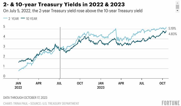
What is the yield curve
telling us right now?
On July 5, 2022, the
yield curve between the two-year and ten-year Treasury notes inverted, and it’s stayed that way since then. It’s
been more than one year since the yield curve inverted, and the economy is
still humming along—unemployment is at 3.8%,
inflation has cooled to 3.7% year-over-year, and consumers are still
spending.
“The U.S. is not in a
recession,” says Garretty. “The labor market
is generating a lot of income for people—they are getting
real gains in their wages…Nobody's happy with these
price increases, but they have the income that allows them to manage it.”
Though it seems like the economy and consumers have yet to
feel the impact of the Fed’s rate hikes—which have risen from near-zero to more than 5% in the
past 18 months—Patterson doesn’t
rule out the possibility of a recession occurring just yet.
“Even though a yield curve of this duration has typically
resulted in a recession in the past, there's good reason to believe a recession
has been delayed for reasons like the housing market remaining resilient and
the strength of the labor market,” says Patterson. “Recession remains our base case. Sometime in 2024.”
Only time will tell whether the recent yield curve
inversion accurately predicts a recession.
“If forecasting recessions was as easy as looking at the
yield curve…you would see a lot more economists
saying things like on November 16 at two o'clock, there will be a recession—it’s clearly not that easy,” says Garretty.
The takeaway
The current inverted yield curve tells us what investors
think will happen to the economy in the future: The Fed will need to cut
interest rates because of a recession. However, when the yield curve inverts,
it’s not always an indicator of an economic downturn—even if it has been in the past.
Regardless of whether a recession occurs, it never hurts to
be ready for one, whether it’s by adding to your
emergency fund or paying off high-interest rate debt.
In
class exercise:
1.
Why
is an inverted yield curve considered a predictor of a future recession?
A) It suggests future
interest rate cuts by the Fed
B) It indicates high
inflation rates
C) It reflects strong
labor market conditions
Answer: A
2.
What is the current status of the yield
curve between the two-year and ten-year Treasury notes?
A) It is upward-sloping
B) It is flat
C) It is inverted
Answer: C
Explanation: As
of July 5, 2022, the yield curve between the two-year and ten-year Treasury
notes is inverted.
3.
What
has been the trend in the U.S. labor market despite the inverted yield curve?
A) High unemployment
rates
B) Stagnant wages
C) Strong job market and
income gains
Answer: C
Explanation:
The labor market is strong, and people are experiencing real gains in their
wages.
4.
How
long does it typically take, according to Garretty and Patterson, for a
recession to occur after the yield curve inverts?
A) 1-3 months
B) 6-12 months
C) 18-24 months
Answer: B
Explanation:
Both Garretty and Patterson estimate it takes around six to 12 months for a
downturn to happen after the yield curve inverts.
5.
What happened in 1966 that is discussed as
an exception egarding the yield curve and recessions?
A) The yield curve
remained inverted without a recession
B) The yield curve
accurately predicted a recession
C) The yield curve did
not invert despite a recession
Answer: A
Explanation: In
1966, there was an inversion of the yield curve that was not followed by a
recession.
6.
Why
does Patterson mention a potential delay in the occurrence of a recession
despite the inverted yield curve?
A) Due to a resilient
housing market
B) Due to low inflation
C) Due to stock market
performance
Answer: A
Explanation:
Patterson suggests that factors like the resilient housing market and the
strength of the labor market may delay a recession.
7.
What has been the trend in the Fed's
benchmark interest rate in the past 18 months, as mentioned in the text?
A) Decreased to
near-zero
B) Remained unchanged
C) Increased to more
than 5%
Answer: C
Explanation:
The article notes that the Fed's benchmark interest rate has risen from
near-zero to more than 5% in the past 18 months.
8.
What is the current stance of the U.S.
economy, according to Garretty?
A) In a recession
B) Generating a lot of
income and experiencing wage gains
C) Experiencing high
inflation and unemployment
Answer: B
Explanation:
Garretty mentions that the U.S. is not in a recession and that the labor
market is generating income for people.
9.
What does the articel suggest about using
the yield curve to predict recessions?
A) It is foolproof and
always accurate
B) It is unreliable and
never accurate
C) It has been a
reliable indicator, but not without exceptions.
Answer: C
Explanation:
While the yield curve has historically predicted recessions, there has been
one false positive in
1966.
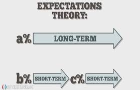
Chapter 6 Interest rate Part II: Term Structure of Interest rate

Question for discussion: If
a% and b% are both known to investors, such as the bank rates, how much is
the future interest rate, such as c%?
(1+a)^N
= (1+b)^m *(1+c)^(N-M)
Either
earning a% of interest rate for N years,
or
b% of interest rate for M years, and then c% of interest rate for (N-M)
years,
investors
should be indifferent. Right?
Then,
(1+a)^N = (1+b)^m *(1+c)^(N-M)è c = ((1+a)^N / (1+b)^m)^(1/(N-M))-1
Or
approximately,
N*a
= M*b +(N-M)*(c)è c = (N*a – M*b) /(N-M)
What Is Expectations Theory (video)
Expectations theory attempts to predict what
short-term interest rates will be in the future based on current
long-term interest rates. The theory suggests that an investor earns the same
amount of interest by investing in two consecutive one-year bond
investments versus investing in one two-year bond today. The theory is also
known as the "unbiased expectations theory.”
Understanding Expectations Theory
The expectations theory aims to help investors make
decisions based upon a forecast of future interest rates. The theory uses
long-term rates, typically from government bonds, to forecast the rate for
short-term bonds. In theory, long-term rates can be used to indicate where
rates of short-term bonds will trade in the future (https://www.investopedia.com/terms/e/expectationstheory.asp)
Expectations Theory
By CHRIS B. MURPHY Updated Apr 21, 2019
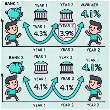
Example of Calculating Expectations Theory
Let's say that the
present bond market provides investors with a two-year bond that
pays an interest rate of 20% while a one-year bond pays an interest rate of
18%. The expectations theory can be used to forecast the interest rate of a
future one-year bond.
- The first step of the
calculation is to add one to the two-year bond’s
interest rate. The result is 1.2.
- The next step is to
square the result or (1.2 * 1.2 = 1.44).
- Divide the result by
the current one-year interest rate and add one or ((1.44 / 1.18) +1 =
1.22).
- To calculate the
forecast one-year bond interest rate for the following year,
subtract one from the result or (1.22 -1 = 0.22 or 22%).
In this example, the investor is earning an equivalent return
to the present interest rate of a two-year bond. If the investor chooses to
invest in a one-year bond at 18% the bond yield for the following year’s bond would need to increase to 22% for this investment
to be advantageous.
- Expectations theory
attempts to predict what short-term interest rates will be in the
future based on current long-term interest rates
- The theory suggests
that an investor earns the same amount of interest
by investing in two consecutive one-year bond investments
versus investing in one two-year bond today
- In theory, long-term rates can be
used to indicate where rates of short-term bonds will trade in the
future
Expectations theory aims to help investors make decisions by
using long-term rates, typically from government bonds, to forecast the rate
for short-term bonds.
Disadvantages of Expectations Theory
Investors should be aware
that the expectations theory is not always a reliable tool. A common problem with using the
expectations theory is that it sometimes overestimates future short-term
rates, making it easy for investors to end up with an inaccurate
prediction of a bond’s yield curve.
Another limitation of the
theory is that many factors impact short-term and long-term bond yields. The
Federal Reserve adjusts interest rates up or down, which impacts bond yields
including short-term bonds. However, long-term yields might not be as
impacted because many other factors impact long-term yields including
inflation and economic growth expectations. As a result, the expectations theory doesn't take into account the outside forces
and fundamental macroeconomic factors that drive interest rates and
ultimately bond yields.
Chapter 6 In class exercise
1 You read
in The Wall Street Journal that 30-day T-bills are currently
yielding 5.5%. Your brother-in-law, a broker at Safe and Sound Securities,
has given you the following estimates of current interest rate premiums:
- Inflation premium = 3.25%
- Liquidity premium = 0.6%
- Maturity risk premium = 1.8%
- Default risk premium = 2.15%
On the
basis of these data, what is the real risk-free rate of return? (answer:
2.25%)
Solution:
General
equation: Rate = r* + Inflation + Default + liquidity + maturity
30-day
T-bills = short term Treasury Security è Default = liquidity = maturity = 0
So
30-day T-bills = 5.5% = r* + inflation =r* + 3.25%
2 The real
risk-free rate is 3%. Inflation is expected to be 2% this year and 4% during
the next 2 years. Assume that the maturity risk premium is zero. What is the
yield on 2-year Treasury securities? What is the yield on 3-year Treasury
securities?(answer: 6%, 6.33%)
Solution:
General
equation: Rate = r* + Inflation + Default + liquidity + maturity
2-year
T-notes = intermediate term Treasury Security è Default = liquidity = 0, maturity=0 as given
Inflation
= average of inflations from year 1 to year 2 = (2% + 4%)/2 = 3%
So
2-year T-notes = r* + inflation = 3% + 3% = 6%
3-year
T-notes = short term Treasury Security è Default = liquidity = 0, maturity=0 as given
Inflation
= average of inflations from year 1 to year 2 = (2% + 4% +4%)/3 = 3.33%
So
2-year T-notes = r* + inflation = 3% + 3.33% = 6.33%
3
A Treasury bond that matures in 10
years has a yield of 6%. A 10-year corporate bond has a yield of 8%. Assume
that the liquidity premium on the corporate bond is 0.5%. What is the default
risk premium on the corporate bond? (answer: 1.5%)
Solution:
General
equation: Rate = r* + Inflation + Default + liquidity + maturity
10 year
T-notes = intermediate term Treasury Security è Default = liquidity = 0, maturity is not zero
So
10-year T-notes = r* + inflation +
maturity = 6%
10 year
corporate bond rate = r* + Inflation +
Default + liquidity + maturity = 8%
Its
liquidity = 0.5%, its maturity = 10-year-notes’ maturity.
Comparing
10 year T-notes and 10 year corporate bonds, we get default = 8%-6%-0.5%=1.5%
|
r* |
inflation |
default |
liquity |
maturity |
|
|
10 - year- T-notes = 6% |
Same |
same |
0 |
0 |
same |
|
10 year corp bonds = 8% |
Same |
same |
? |
1.50% |
same |
4 The real risk-free rate is 3%, and inflation
is expected to be 3% for the next 2 years. A 2-year Treasury
security yields 6.2%. What is the maturity risk premium for the 2-year
security? (answer: 0.2%)
General
equation: Rate = r* + Inflation + Default + liquidity + maturity
2-year
T-notes = intermediate term Treasury Security è Default = liquidity = 0, maturity=?
2-year
T-notes = 6.2% = r* + inflation + maturity = 3% + 3% + maturity
5 One-year Treasury securities yield 5%. The market
anticipates that 1 year from now, 1-year Treasury securities will yield 6%.
If the pure expectations theory is correct, what is the yield today for
2-year Treasury securities? (answer: 5.5%)

Or,

Real Interest rate in the US from 2000-2022
https://fred.stlouisfed.org/series/REAINTRATREARAT1YE
Three Month
T-Bill rate (a proxy of the risk free rate)

https://www.cnbc.com/quotes/US3M

|
Year |
Jan |
Feb |
Mar |
Apr |
May |
Jun |
Jul |
Aug |
Sep |
Oct |
Nov |
Dec |
Ave |
|
2023 |
6.4 |
6 |
5 |
4.9 |
4 |
3 |
3.2 |
3.7 |
3.7 |
3.2 |
3.1 |
3 |
4 |
|
2022 |
7.5 |
7.9 |
8.5 |
8.3 |
8.6 |
9.1 |
8.5 |
8.3 |
8.2 |
7.7 |
7.1 |
6.5 |
8 |
|
2021 |
1.4 |
1.7 |
2.6 |
4.2 |
5 |
5.4 |
5.4 |
5.3 |
5.4 |
6.2 |
6.8 |
7 |
4.7 |
|
2020 |
2.5 |
2.3 |
1.5 |
0.3 |
0.1 |
0.6 |
1 |
1.3 |
1.4 |
1.2 |
1.2 |
1.4 |
1.2 |
|
2019 |
1.6 |
1.5 |
1.9 |
2 |
1.8 |
1.6 |
1.8 |
1.7 |
1.7 |
1.8 |
2.1 |
2.3 |
1.8 |
|
2018 |
2.1 |
2.2 |
2.4 |
2.5 |
2.8 |
2.9 |
2.9 |
2.7 |
2.3 |
2.5 |
2.2 |
1.9 |
2.4 |
|
2017 |
2.5 |
2.7 |
2.4 |
2.2 |
1.9 |
1.6 |
1.7 |
1.9 |
2.2 |
2 |
2.2 |
2.1 |
2.1 |
|
2016 |
1.4 |
1 |
0.9 |
1.1 |
1 |
1 |
0.8 |
1.1 |
1.5 |
1.6 |
1.7 |
2.1 |
1.3 |
|
2015 |
-0.1 |
0 |
-0.1 |
-0.2 |
0 |
0.1 |
0.2 |
0.2 |
0 |
0.2 |
0.5 |
0.7 |
0.1 |
|
2014 |
1.6 |
1.1 |
1.5 |
2 |
2.1 |
2.1 |
2 |
1.7 |
1.7 |
1.7 |
1.3 |
0.8 |
1.6 |
|
2013 |
1.6 |
2 |
1.5 |
1.1 |
1.4 |
1.8 |
2 |
1.5 |
1.2 |
1 |
1.2 |
1.5 |
1.5 |
|
2012 |
2.9 |
2.9 |
2.7 |
2.3 |
1.7 |
1.7 |
1.4 |
1.7 |
2 |
2.2 |
1.8 |
1.7 |
2.1 |
|
2011 |
1.6 |
2.1 |
2.7 |
3.2 |
3.6 |
3.6 |
3.6 |
3.8 |
3.9 |
3.5 |
3.4 |
3 |
3.2 |
|
2010 |
2.6 |
2.1 |
2.3 |
2.2 |
2 |
1.1 |
1.2 |
1.1 |
1.1 |
1.2 |
1.1 |
1.5 |
1.6 |
|
2009 |
0 |
0.2 |
-0.4 |
-0.7 |
-1.3 |
-1.4 |
-2.1 |
-1.5 |
-1.3 |
-0.2 |
1.8 |
2.7 |
-0.4 |
|
2008 |
4.3 |
4 |
4 |
3.9 |
4.2 |
5 |
5.6 |
5.4 |
4.9 |
3.7 |
1.1 |
0.1 |
3.8 |
|
2007 |
2.1 |
2.4 |
2.8 |
2.6 |
2.7 |
2.7 |
2.4 |
2 |
2.8 |
3.5 |
4.3 |
4.1 |
2.8 |
|
2006 |
4 |
3.6 |
3.4 |
3.5 |
4.2 |
4.3 |
4.1 |
3.8 |
2.1 |
1.3 |
2 |
2.5 |
3.2 |
|
2005 |
3 |
3 |
3.1 |
3.5 |
2.8 |
2.5 |
3.2 |
3.6 |
4.7 |
4.3 |
3.5 |
3.4 |
3.4 |
|
2004 |
1.9 |
1.7 |
1.7 |
2.3 |
3.1 |
3.3 |
3 |
2.7 |
2.5 |
3.2 |
3.5 |
3.3 |
2.7 |
|
2003 |
2.6 |
3 |
3 |
2.2 |
2.1 |
2.1 |
2.1 |
2.2 |
2.3 |
2 |
1.8 |
1.9 |
2.3 |
|
2002 |
1.1 |
1.1 |
1.5 |
1.6 |
1.2 |
1.1 |
1.5 |
1.8 |
1.5 |
2 |
2.2 |
2.4 |
1.6 |
|
2001 |
3.7 |
3.5 |
2.9 |
3.3 |
3.6 |
3.2 |
2.7 |
2.7 |
2.6 |
2.1 |
1.9 |
1.6 |
2.8 |
|
2000 |
2.7 |
3.2 |
3.8 |
3.1 |
3.2 |
3.7 |
3.7 |
3.4 |
3.5 |
3.4 |
3.4 |
3.4 |
3.4 |
https://www.usinflationcalculator.com/inflation/current-inflation-rates/#google_vignette
Chapter 6 – Assignments –
(FYI: Videos: www.jufinance.com/video/fin435_chapter_6_case_video_1.mp4 (1/18/2023)
www.jufinance.com/video/fin435_chapter_6_case_video_2.mp4 (1/23/2023))
·
Chapter six case study (due with
  first mid term exam)
·
Critical thinking question 1: What factors contributed
to the shifts in yield curve shapes in 2023?
·
Critical thinking question 2: Do you think we will
enter a recession as predicted by the inverted yield curve?
·
Critical
thinking question 3: Do you endorse the notion of the Federal Reserve lowering interest
rates in 2024? Why or why not?
Chapter 7 Bond Valuation

For discussion: https://jufinance.com/risk_tolerance.html
|
Bond Type |
Characteristics |
Suitability |
Risk |
|
Short-Term Bonds |
Quick maturity, Low risk,
Lower returns |
Conservative, Need
liquidity |
Reinvestment Risk |
|
Long-Term Bonds |
Higher returns, High
risk |
Long-term, High risk
tolerance |
Default Risk; Market
interest rate risk |
|
Corporate Bonds |
Higher yields, Higher risk,
Company influence |
Seeking returns, Accepting
higher risk |
Default Risk; Market interest rate risk (assuming long
maturity) |
|
Treasury Securities |
Low risk, Steady income,
Different maturities |
Conservative, Stable income
requirement |
Market interest rate risk
(assuming long maturity) |
|
Municipal Bonds |
Tax advantages, Credit
risk |
Tax-efficient income, Higher
tax bracket |
Default Risk; Market interest rate risk (assuming long
maturity) |
·
Among the aforementioned bonds, do you have a preference? If so, what
factors influence your choice?

Outlook
for Investing in Bonds in 2024
After starting the year recommending that investors focus on
the middle of the yield curve, we began to advise investors to lengthen their
duration in our midyear bond
market update. According to our forecasts, we continue to think investors will be best served in longer-duration bonds and locking in the currently high interest
rates. https://www.morningstar.com/markets/where-invest-bonds-2024
Market data website:
FINRA: https://www.finra.org/finra-data/fixed-income (FINRA bond
market data)

Relationship
between bond prices and interest rates (Khan academy)
In class exercise
1)
What is the face value (par value) of the bond?
a. $500
b. $1,000
c. $1,500
2)
How often are coupon payments made on the bond?
a. Annually
b. Semi-annually
c. Quarterly
3)
If the bond has a two-year maturity, what is the total number of
coupon payments made over its life?
a. 2
b. 4
c. 6
4)
If interest rates rise after the bond is purchased, what happens
to its price?
a. Increases
b.
Decreases
c. Remains unchanged
5)
If interest rates go down, what is the likely impact on the
bond's price?
a.
Increases
b. Decreases
c. Remains unchanged
6)
For a zero-coupon bond with a face value of $1,000 and a
two-year maturity, what is the price if the expected return is 10% per year?
a. $823
b. $1,000
c. $1,100
7)
In the scenario of increased expectations, if the expected
return is now 15% for the same zero-coupon bond, what happens to its price?
a. Increases
b.
Decreases
c. Remains unchanged
8)
If the expected return decreases to 5% for the same zero-coupon
bond, what is the new price?
a. $822
b. $905
c. $1,000
9)
What does a bond trading at a premium mean?
a. Its price is below par
b. Its price is
above par
c. Its price is equal to par
10)
What does a bond trading at a discount mean?
a. Its price is
below par
b. Its price is above par
c. Its price is equal to par
11)
If interest rates are lower than expected, how does it affect
the price of a bond?
a. Increases
b. Decreases
c. Increases
12)
What is the primary reason for a bond trading at a discount?
a. High coupon rate
b. Low market interest rates
c. Low coupon
rate
13)
In the context of bond pricing, what is the present value?
a. Future value of cash flows
b. Current value
of future cash flows
c. Face value of the bond
14)
Why does the price of a bond decrease when interest rates rise?
a. Increase in coupon payments
b. Decrease in market expectations
c. Decrease in
present value of future cash flows
15)
What does a bond trading at par mean?
a. Its price is below par
b. Its price is above par
c. Its price is
equal to par
Reading
material:
·
Interest rate risk — When
Interest rates Go up, Prices of Fixed-rate Bonds Fall, issued by SEC at https://www.sec.gov/files/ib_interestraterisk.pdf
·

·
Higher market interest rates è lower fixed-rate bond prices è higher fixed-rate bond
yields
·
Lower fixed-rate bond coupon rates
è higher interest rate risk
·
Higher fixed-rate bond coupon rates è lower interest rate risk
·
Lower market interest rates è higher fixed-rate bond prices è lower fixed-rate bond yields èhigher interest rate risk to rising market
interest rates
·
Longer maturity è higher interest rate risk è higher coupon rate
·
Shorter maturity è lower interest rate risk è lower coupon rate
From https://www.sec.gov/files/ib_interestraterisk.pdf
In class exercise: True / False
1)
Higher
market interest rates lead to higher fixed-rate bond yields.
True
Explanation: Higher market interest rates result in lower fixed-rate bond prices and, consequently, higher fixed-rate bond yields.
2)
Lower
fixed-rate bond coupon rates decrease interest rate risk.
False
Explanation: When a bond has a lower fixed-rate coupon, the bondholder receives less interest income. In a rising interest rate environment, new bonds with higher coupon rates become more attractive to investors, leading to a decrease in the market value of existing bonds with lower coupon rates. Therefore, lower fixed-rate bond coupon rates make the bond more sensitive to changes in interest rates, resulting in higher interest rate risk.
3)
Higher
fixed-rate bond coupon rates lead to higher interest rate risk.
False
Explanation: Higher coupon rates lower interest rate risk for fixed-rate bonds. See above for further explanation.
4)
Lower
market interest rates result in higher fixed-rate bond yields.
False
Explanation: Lower market interest rates lead to higher fixed-rate bond prices and lower fixed-rate bond yields.
5)
Longer
maturity is associated with lower interest rate risk and a lower coupon rate.
False
Explanation: Longer maturity is associated with higher interest rate risk and a higher coupon rate. In terms of coupon rates, there is a general tendency for longer-maturity bonds to have higher coupon rates. This is because investors typically demand higher compensation for the increased interest rate risk associated with longer-term investments.
6)
Shorter
maturity reduces interest rate risk and increases the coupon rate.
False
Explanation: Shorter maturity is associated with lower interest rate risk and a lower coupon rate.
7)
Rising
market interest rates decrease fixed-rate bond prices and increase interest
rate risk.
True
Explanation: Rising market interest rates lead to lower fixed-rate bond prices and higher interest rate risk.
8)
Lower
fixed-rate bond coupon rates result in higher fixed-rate bond prices.
False
Explanation: Lower fixed-rate bond coupon rates generally result in lower demand and, consequently, lower bond prices, since when a bond has a lower coupon rate, it becomes less attractive to investors seeking higher yields. As a result, the bond's market price tends to decrease.
9)
Shorter
maturity is associated with higher interest rate risk and a higher coupon
rate.
False.
Explanation: Shorter maturity is associated with lower interest rate risk, not higher. When a bond has a shorter maturity, it means that the time until the bond's principal is repaid is shorter. In such cases, changes in interest rates have a lesser impact on the bond's price. The correct statement should be “Shorter maturity is associated with lower interest rate risk and a lower coupon rate”.
Bond Pricing Excel Formula
To calculate bond price in EXCEL (annual coupon
bond):
Price=abs(pv(yield to maturity, years left to maturity, coupon
rate*1000, 1000)
To calculate yield to maturity (annual coupon bond)::
Yield to maturity = rate(years left to maturity, coupon rate
*1000, -price, 1000)
To calculate bond price (semi-annual coupon bond):
Price=abs(pv(yield to maturity/2, years left to maturity*2,
coupon rate*1000/2, 1000)
To calculate yield to maturity (semi-annual coupon bond):
Yield to maturity = rate(years left to maturity*2, coupon
rate *1000/2, -price, 1000)*2
In Class Exercise (could be used to prepare for the
first midterm exam)
Excel Solution Video-Part 1 Video-Part 2
1.
AAA firm’ bonds will mature in eight years, and coupon is $65.
YTM is 8.2%. Bond’s market value? ($903.04, abs(pv(8.2%, 8, 65, 1000))
·
Rate 8.2%
·
Nper 8
·
Pmt 65
·
Pv ?
·
FV 1000
2. AAA firm’s bonds’ market value is $1,120, with
15 years maturity and coupon of $85. What is YTM? (7.17%,
rate(15, 85, -1120, 1000))
·
Rate ?
·
Nper 15
·
Pmt 85
·
Pv -1120
·
FV 1000
3. Sadik
Inc.'s bonds currently sell for $1,180 and have a par value of
$1,000. They pay a $105 annual coupon
and have a 15-year maturity, but they can be called in 5 years at
$1,100. What is their yield
to call (YTC)? (7.74%, rate(5, 105, -1180, 1100)) What is
their yield to maturity (YTM)? (8.35%, rate(15,
105, -1180, 1000))
·
Rate ?
·
Nper 15
·
Pmt 105
·
Pv -1180
·
FV 1000
4. Malko
Enterprises’ bonds currently sell for $1,050. They have a 6-year
maturity, an annual coupon of $75, and a par value of $1,000. What
is their current yield? (7.14%,
75/1050)
5. Assume
that you are considering the purchase of a 20-year, noncallable bond with an
annual coupon rate of 9.5%. The bond has a face value of $1,000,
and it makes semiannual interest payments. If you require an 8.4%
nominal yield to maturity on this investment, what is the maximum price you
should be willing to pay for the bond? ($1,105.69, abs(pv(8.4%/2, 20*2, 9.5%*1000/2, 1000)) )
·
Rate 8.4%/2
·
Nper 20*2
·
Pmt 95/2
·
Pv ?
·
FV 1000
6. Grossnickle
Corporation issued 20-year, non-callable, 7.5% annual coupon bonds at their
par value of $1,000 one year ago. Today, the market interest rate
on these bonds is 5.5%. What is the current price of the bonds,
given that they now have 19 years to maturity? ($1,232.15, abs(pv(5.5%, 19, 75, 1000)))
·
Rate 7.5%/2
·
Nper 19
·
Pmt 75
·
Pv ?
·
FV 1000
7. McCue
Inc.'s bonds currently sell for $1,250. They pay a $90 annual coupon, have a
25-year maturity, and a $1,000 par value, but they can be called in 5 years
at $1,050. Assume that no costs other than the call premium would
be incurred to call and refund the bonds, and also assume that the yield curve is horizontal, with
rates expected to remain at current levels on into the
future. What is the difference between this bond's YTM and its
YTC? (Subtract the YTC from the YTM; it is possible to get a
negative answer.) (2.62%, YTM = rate(25, 90,
-1250, 1000), YTC = rate(5, 90, -1250, 1050))
·
Rate ? ------------ ?
·
Nper 25 ------------- 5
·
Pmt 90 ------------ 90
·
Pv -1250 ------------ -1250
·
FV 1000 ------------ 1000
8. Taussig
Corp.'s bonds currently sell for $1,150. They have a 6.35% annual
coupon rate and a 20-year maturity, but they can be called in 5 years at
$1,067.50. Assume that no costs other than the call premium would
be incurred to call and refund the bonds, and also assume that the yield
curve is horizontal, with rates expected to remain at current levels on into
the future. Under these conditions, what rate of return should an
investor expect to earn if he or she purchases these bonds? (4.2%, rate(5, 63.5, -1150, 1067.5))
9. A
25-year, $1,000 par value bond has an 8.5% annual payment
coupon. The bond currently sells for $925. If the yield
to maturity remains at its current rate, what will the price be 5 years from
now? ($930.11, rate(25, 85, -925, 1000),
abs(pv( rate(25, 85, -925, 1000), 20, 85, 1000))
Assignments of Chapter 7:
1)
Chapter 7 Case Study – Due
with first midterm exam (updated)
Case study video in class 1/30/2024
(video. Thanks, Chris)
2)
Critical
Thinking Challenge –
Just choose one of the two questions as follows from https://www.cnbc.com/2023/11/01/fixed-income-back-in-the-spotlight-how-investors-can-take-advantage.html:
Option 1 -
The Impact of Rising Interest Rates on Bond Investments:
a.
Describe the recent shift in interest
rates and its impact on bond investments.
b.
Discuss the reasons behind the
dramatic increase in interest rates and how this shift has affected the bond
market.
Option 2 - The Role of Active
Fixed-Income Management in Volatile Markets:
a. Discuss the importance of
adopting an active approach to fixed-income management in the current
volatile market.
b. Explore how an active approach
allows for better returns and the flexibility to navigate challenging market
conditions.
3)
A quick quiz on the conceptual
comprehension of the bond chapter (FYI only, not required):
Bond Pricing Formula (FYI)


![]()
Bond Pricing Excel Formula
To calculate bond price in EXCEL (annual
coupon bond):
Price=abs(pv(yield to maturity, years left to maturity,
coupon rate*1000, 1000)
To calculate yield to maturity (annual coupon bond)::
Yield to maturity = rate(years left to maturity, coupon
rate *1000, -price, 1000)
To calculate bond price (semi-annual coupon bond):
Price=abs(pv(yield to maturity/2, years left to
maturity*2, coupon rate*1000/2, 1000)
To calculate yield to maturity (semi-annual coupon
bond):
Yield to maturity = rate(years left to maturity*2,
coupon rate *1000/2, -price, 1000)*2
Bond Duration Calculator
(FYI)
https://exploringfinance.com/bond-duration-calculator/
Op-ed: Fixed income is back
in the spotlight. Here’s how investors can take advantage
PUBLISHED WED, NOV 1
2023 9:00 AM EDT Christopher
Gunster, head of fixed income at Fidelis Capital
KEY POINTS
·
In recent quarters, we have
witnessed a dramatic shift higher in interest rates, a move that investors
should not fear but embrace. Bonds are now all the rage.
·
The current real yield on a
10-year Treasury is approaching 2.5%, a level that should excite bond
investors.
·
Return expectations are the
highest in years and, although markets could remain volatile, now is the
appropriate time to reassess your portfolio and consider an increase in your
fixed-income allocation.
Fixed-income investing is entering an exciting new era, and
investors should take notice. Decades
of low interest rates, engineered by global central banks, have suppressed
the bond market’s ability to generate attractive and
reliable returns.
But in recent quarters, we have witnessed a dramatic shift
higher in interest rates, a move that investors should not fear but embrace.
Bonds are now all the rage in investing circles and, although not as trendy
as Taylor Swift, their popularity has certainly risen in recent months
alongside interest rates.
Interest rates have increased dramatically since the beginning
of 2022. As an example, the yield-to-maturity on the benchmark U.S. 10-year
Treasury
is now nearing 5%, up
over 3.30%.
The yield on the 10-year and
other Treasury bonds is now the highest since the onset of the Great
Financial Crisis in 2007. In addition
to the rise in nominal interest rates, we have also experienced a similar
increase in real interest rates (rates adjusted for inflation).
If we use market-derived, forward-looking expectations of
inflation to adjust nominal yields, the current real yield on a 10-year
Treasury is approaching 2.5%, a level that should excite bond investors.

Granted, the journey to
higher yields has been painful to bond investors. In 2022, the total return of the Bloomberg Aggregate Bond
Index, a broad universe of U.S. taxable bonds, posted a return of -13.01%
(according to Bloomberg as of Dec. 31, 2022), the worst calendar year
performance for this index since its inception in 1976.
Other bond market sectors experienced similar distress, but with
the pain comes the gain. Higher rates
can now provide more total return and more stability in returns going
forward.
When calculating fixed-income returns for most bonds, there
are two components: price return and income return.
First time seeing Treasury yield move like this in 20-year
career, says Exante Data’s Jens Nordvig
At the start of 2022, there was little income being generated
from high-quality bonds. The negative total returns for the year were driven
by large price declines with a small positive contribution from income.
As an example, the Bloomberg Aggregate Bond Index posted a
price return of -15.3% and an income return of +2.3%. However, the
yield-to-maturity on the Bloomberg Aggregate Index is now 5.64% (according to
Bloomberg as of Oct. 17, 2023), over 3.5% higher than the beginning of 2022.
As a result, we would expect a much larger positive
contribution to future returns from income and a less negative contribution
from price return.
How can an investor take
advantage of the higher-yield environment?
We would suggest that
investors reassess their current bond allocation and marginally increase
their exposure in a manner consistent with their portfolio’s
current position, investment objectives and risk tolerance.
While we are not calling the top in near-term rate movements,
we do believe we are entering more of a range-bound yield market for longer
maturity bonds. This is consistent with our expectations of no additional
rate hikes from the Federal Reserve this cycle and a continued decline in
near-term inflation.
To efficiently capture the higher yields, we would advise a modest increase in longer-dated
maturity bonds as well as an allocation to shorter maturity bonds in a
barbell approach, while avoiding intermediate maturity where possible.
Given the inverted shape of
the yield curve, a barbell approach can help maximize the overall yield of
the portfolio and provide additional return should long-end rates move lower.
For non-taxable or investors
that are not tax-sensitive, we would prefer the use of higher-quality
corporate bonds, as we believe the market has not appropriately priced the
risk of a potential recession in lower-quality bonds.
Additionally, the agency
mortgage-backed securities market is a high-quality sector for investors to
consider. Year to date, this sector
has underperformed other investment grade sectors and now offers an
attractive risk-return profile.
For those investors in
high-income tax brackets, municipal bonds are attractive. Similar to our view
on taxable bonds, we would recommend a bias toward higher-quality bonds as a
potential recession could negatively impact lower-rated municipalities.
While we currently favor
municipal bonds for those high-tax investors, we would not eliminate
corporate bonds or other taxable securities from consideration. Certain
market conditions can favor taxable bonds on an after-tax, risk-adjusted
basis.
It’s important that investors select a
manager who can take advantage of those opportunities when they arise to
create a tax-efficient portfolio.
To the extent that interest rates move significantly higher,
counter to our expectations, we would view this as an opportunity for
investors to lock in even higher yields for longer. Under such a scenario, we
would not expect a repeat of 2022 bond market returns.
We estimate that interest rates would have to increase by
0.70% to 1.00% before forward-looking 12-month total returns would turn
negative for the major bond indexes.
We have little doubt that
the heightened level of market volatility will continue into 2024.
Opportunities present themselves when market volatility increases.
To that end, we recommend an
active approach to fixed-income management. Having the flexibility to successfully navigate and benefit
during challenging markets allows for better returns.
It is a new dawn for bonds and fixed-income investors. Return
expectations are the highest in years and, although markets could remain
volatile, now is the appropriate time to reassess your portfolio and consider
an increase in your fixed-income allocation.
— By Christopher Gunster, head of fixed income at Fidelis
Capital
In class exercise
1. What is the key
point emphasized in the op-ed regarding fixed income?
a.
Fixed income is losing popularity
b.
Investors should fear the recent shift in interest rates
c.
Fixed income is back in the spotlight
Answer: c.
Explanation:
The op-ed highlights the resurgence of fixed income in recent quarters.
2. What
is the current real yield on a 10-year Treasury, as mentioned in the op-ed?
a. 3.5%
b. 2.5%
c.
5.64%
Answer: b.
Explanation:
The op-ed states that the current real yield on a 10-year Treasury is
approaching 2.5%.
3. How
did the Bloomberg Aggregate Bond Index perform in 2022, according to the
op-ed?
a.
Positive return
b.
-15.3% return
c.
-13.01% return
Answer: c.
Explanation:
The op-ed mentions a negative total return of -13.01% for the Bloomberg
Aggregate Bond Index in 2022.
4. What
is suggested as a strategy to take advantage of the higher-yield environment?
a.
Increase bond exposure
b.
Reduce bond exposure
c.
Maintain the current bond allocation
Answer: a.
Explanation:
The op-ed suggests reassessing and marginally increasing bond exposure.
5. What
type of bond allocation is recommended for non-taxable or tax-insensitive
investors?
a.
Corporate bonds
b.
Municipal bonds
c.
Agency mortgage-backed securities
Answer: a.
Explanation:
Higher-quality corporate bonds are preferred for non-taxable or tax-insensitive
investors.
6. What
does the op-ed recommend for investors in high-income tax brackets?
a.
Municipal bonds
b.
Corporate bonds
c.
Agency mortgage-backed securities
Answer: a.
Explanation:
Municipal bonds are recommended for investors in high-income tax brackets.
7. What
does the op-ed suggest about the agency mortgage-backed securities market?
a. It
is not recommended for investment
b. It
has outperformed other investment grade sectors
c. It
is a high-risk sector
Answer: b.
Explanation:
The op-ed mentions that this sector has underperformed other investment grade
sectors.
8. What
is the recommended approach for capturing higher yields in a portfolio?
a.
Focus on intermediate maturity bonds
b.
Invest only in longer-dated maturity bonds
c. Use a
barbell approach with longer and shorter maturity bonds
Answer: c.
Explanation:
A barbell approach is advised to maximize overall portfolio yield.
9. What
is recommended for investors to consider in response to market volatility,
according to the op-ed?
a.
Adopt a passive approach
b.
Increase exposure to stocks
c. Take
an active approach to fixed-income management
Answer: c.
Explanation:
The op-ed recommends an active approach to benefit during challenging
markets.
10.
What is described as the current state of return expectations for bonds and
fixed-income investors?
a. The
highest in years
b. The
lowest in years
c.
Stable and predictable
Answer: a.
Explanation:
The op-ed suggests that return expectations are the highest in years.
11.
What is the op-ed's suggestion regarding reassessing portfolios in the
current environment?
a. It
is not necessary to reassess portfolios
b.
Portfolios should be reassessed and fixed-income allocation increased
c.
Portfolios should be reassessed, but fixed-income allocation should be
decreased
Answer: b.
Explanation:
The op-ed suggests reassessing portfolios and considering an increase in
fixed-income allocation.
Chapter 8 Risk and Return
Equations
1. Expected return and standard deviation
Given
a probability distribution of returns, the expected return can be calculated
using the following equation:

where
- E[R] = the
expected return on the stock,
- N = the
number of states,
- pi =
the probability of state i, and
- Ri =
the return on the stock in state i.
Given
an asset's expected return, its variance can be calculated using the
following equation:

where
- N = the
number of states,
- pi =
the probability of state i,
- Ri =
the return on the stock in state i, and
- E[R] = the
expected return on the stock.
The
standard deviation is calculated as the positive square root of the variance.

http://www.zenwealth.com/businessfinanceonline/RR/MeasuresOfRisk.html
2. Two stock portfolio equations:
![]()
W1 and W2 are the
percentage of each stock in the portfolio.

Portfolio Variance Part 1
(youtube)
![]()
- r12 =
the correlation coefficient between the returns on stocks 1 and 2,
- s12 =
the covariance between the returns on stocks 1 and 2,
- s1 =
the standard deviation on stock 1, and
- s2 =
the standard deviation on stock 2.
![]()
- s12 =
the covariance between the returns on stocks 1 and 2,
- N = the
number of states,
- pi =
the probability of state i,
- R1i =
the return on stock 1 in state i,
- E[R1]
= the expected return on stock 1,
- R2i =
the return on stock 2 in state i, and
- E[R2]
= the expected return on stock 2.
3.. Historical returns
Holding period return (HPR) = (Selling price – Purchasing price
+ dividend)/ Purchasing price
4. CAPM model
· What Is the Capital Asset Pricing Model?
The Capital Asset Pricing Model (CAPM)
describes the relationship between systematic risk and expected
return for assets, particularly stocks. CAPM is widely used throughout
finance for pricing risky securities and generating expected
returns for assets given the risk of those assets and cost of capital.
Ri = Rf + βi
*( Rm - Rf) ------ CAPM model
Ri = Expected return
of investment
Rf =
Risk-free rate
βi =
Beta of the investment
Rm =
Expected return of market
(Rm -
Rf) = Market risk premium
· What is Beta? Where to find Beta?

· SML – Security Market Line

RISK and Return General Template
In Class Exercise Video
|
1.
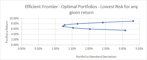
How to achieve the best investment results (low risk, high return)
(SOLUTION,
updated FYI) |
|||||
|
- Modern
Portfolio Theory |
|||||
|
Three stock portfolio: A, B,
C |
|||||
|
Year |
A |
B |
C |
|
|
|
1 |
10% |
4% |
12% |
|
|
|
2 |
5% |
6% |
5% |
|
|
|
3 |
4% |
8% |
7% |
|
|
|
4 |
7% |
10% |
8% |
|
|
|
5 |
1% |
5% |
14% |
|
|
Assuming
you have $10,000, how should you allocate funds among the three stocks to
create an optimal portfolio with the highest return and lowest risk?
Steps
1.
Mean, risk for each stock
2.
Correlation between stocks: 3 correlations
3. Set
it up as a portfolio and get portfolio's mean and risk
Portfolio Return = w1*r1
+ w2*r2 + w3*r3
where: w1, w2, w3
are the weights of each stock in the portfolio, and r1,
r2, r3 are the returns of each stock in the
portfolio.
Portfolio Standard Deviation:
Portfolio Standard Deviation = sqrt(w12*σ12+ w22*σ22+ w32*σ32 + 2*w1*w2*ρ12*σ1*σ2 + 2*w1*w3*ρ13*σ1*σ3 + 2*w2*w3*ρ23*σ2*σ3)
where: σ1,
σ2,
σ3
are the standard deviations of each stock
in the portfolio. ρ12, ρ13, ρ23 are correlation coefficients between the stock returns. They
represent the pairwise correlations between the stocks in the portfolio.
For example, ρ12 represents
the correlation coefficient between the returns of stock 1 and stock 2, ρ23 represents
the correlation coefficient between the returns of stock 2 and stock.
4. Use
solver to find lowest risk (standard deviation) for any given return.
2. An investor currently holds the following portfolio: He invested
30% of the fund in Apple with Beta equal 1.1. He also invested 40% in GE with
Beta equal 1.6. The rest of his fund goes to Ford, with Beta equal 2.2. Use
the above information to answer the following questions.
1) The beta for the portfolio is? (1.63)
Solution:
0.3*1.1+0.4*1.6+(1-0.3-0.4)*2.2=1.63(weighted average of beta)
3.
The three month
Treasury bill rate (this is risk free rate) is 2%. S&P500 index return is
10% (this is market return). Now calculate the portfolio’s
return. 15.04%
Solution:
0.3*1.1+0.4*1.6+(1-0.3-0.4)*2.2=1.63--- This is beta and then
plug into the CAPM.
Return = 2% + 1.63*(10%-2%) = 15.04%
Refer to the following graph. The three month
Treasury bill rate (this is risk free rate) is 2%. S&P500 index return is
10% (this is market return).
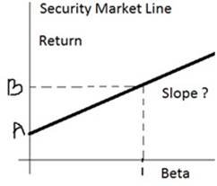
1.
What is the value of A? 2%
Solution:
This is the intercept of the SML
2.
What is the value of B? 10%
Solution:
B is the market return, so 10%, since Beta =1
3.
How much is the slope of the above security market line? 8%
Solution:
Slope = rise/run = (10%-2%)/(1-0), just compare risk free rate
(Beta=0) and market return (beta=1)
4.
Your uncle bought Apple in January, year 2000 for $30. The
current price of Apple is $480 per share. Assume there are no dividend ever
paid. Calculate your uncle’s holding period return. 15 times
Solution:
Holding period return = (480-30)/30 =1500%=15
times
5.
Your current portfolio’s BETA is about 1.2. Your total
investment is worth around $200,000. You uncle just gave you $100,000 to
invest for him. With this $100,000 extra funds in hand, you plan to invest
the whole $100,000 in additional stocks to increase your whole portfolio’s
BETA to 1.5 (Your portfolio now worth $200,000 plus $100,000). What is the
average BETA of the new stocks to achieve your goal? (hint: write down the
equation of the portfolio’s Beta first) 2.10
Solution:
Total amount = 200000 + 100000=300000
New portfolio beta = 1.2*200000/300000 +
X*(100000/300000) = 1.5 è X=2.1
7.
Years Market
r Stock
A Stock
B
1 3% 16% 5%
2 -5% 20% 5%
3 1% 18% 5%
4 -10% 25% 5%
5 6% 14% 5%
· Calculate the average returns of the market r
and stock A and stock B. (Answer:
-1%, 18.6%, 5%)
· Calculate the standard deviations of the
market, stock A, & stock B (Answer:
6.44%, 4.21%; 0 )
· Calculate the correlation of stock market r
and stock a. (Answer: -0.98)
· Assume you invest 50% in stock A and 50% in
stock B. Calculate the average return and the standard deviation of the
portfolio. (Answer: 11.8%; 2.11%)
Calculate beta of
stock A and beta of stock B, respectively (Answer:
-0.64, 0)
Solution of Question 7,
or refer to https://www.jufinance.com/portfolio/
9. Another practice quiz
– FYI only
What Is
the Capital Asset Pricing Model?
The Capital Asset Pricing Model (CAPM)
describes the relationship between systematic risk and expected
return for assets, particularly stocks. CAPM is widely used throughout
finance for pricing risky securities and generating expected
returns for assets given the risk of those assets and cost of capital.
Ri = Rf + βi
*( Rm - Rf) ------ CAPM model
Ri = Expected return
of investment
Rf =
Risk-free rate
βi =
Beta of the investment
Rm =
Expected return of market
(Rm -
Rf) = Market risk premium
Investors
expect to be compensated for risk and the time value of money.
The risk-free rate in the CAPM formula accounts for the time value
of money. The other components of the CAPM formula account for the investor
taking on additional risk.
The beta of
a potential investment is a measure of how much risk the investment will add
to a portfolio that looks like the market. If a stock is riskier than the
market, it will have a beta greater than one. If a stock has a beta of less
than one, the formula assumes it will reduce the risk of a portfolio.
A
stock’s beta is then multiplied by the market risk premium, which is the
return expected from the market above the risk-free rate. The risk-free rate
is then added to the product of the stock’s beta and the market risk
premium. The result should give an investor the required
return or discount rate they can use to find the value of an
asset.
The
goal of the CAPM formula is to evaluate whether a stock is fairly valued when
its risk and the time value of money are compared to its expected return.
For example, imagine an investor is
contemplating a stock worth $100 per share today that pays a 3% annual
dividend. The stock has a beta compared to the market of 1.3, which means it
is riskier than a market portfolio. Also, assume that the risk-free rate is
3% and this investor expects the market to rise in value by 8% per year.
The expected return of the stock based
on the CAPM formula is 9.5%.
The
expected return of the CAPM formula is used to discount the expected
dividends and capital appreciation of the stock over the expected holding
period. If the discounted value of those future cash flows is equal to $100
then the CAPM formula indicates the stock is fairly valued relative to risk.
(https://www.investopedia.com/terms/c/capm.asp)
Finding
Beta Value (https://finance.zacks.com/stock-beta-value-8004.html)
The current beta
value of a company stock is provided for free by many online financial news
services, including Morningstar, Google Finance and Yahoo Finance. Online
brokerage services provide more extensive tracking of a company's beta
measurements, including historical trends. Beta is sometimes listed under
"market data" or other similar headings, as it describes past
market performance. A stock with a beta of 1.0 has the same price volatility
as the market index, meaning if the market gains, the stock makes gains at
the same rate. A stock with a beta of greater than 1.0 is riskier and has
greater price fluctuations, while stocks with beta values of less than 1.0
are steadier and generally larger companies.
Examples of Beta
Beta is often
measured against the S&P 500 index. An
S&P 500 stock with a beta of 2.0 produced a 20 percent increase in
returns during a period of time when the S&P 500 Index grew only 10
percent. This same measurement also means the stock would lose 20 percent
when the market dropped by only 10 percent. High beta values, including those
more than 1.0, are volatile and carry more risk along with greater potential
returns. The measurement doesn't distinguish between upward and downward
movements. Investing Daily notes that investors try to use stocks with high
beta values to quickly recoup their investments after sharp market losses.
Small-Cap Stocks
Beta values are useful to
evaluate stock prices of smaller companies. These small-capitalization stocks
are attractive to investors because their price volatility can promise
greater returns, but Market Watch recommends only buying small-cap stocks
with beta values of less than 1.0. The beta value is also a component of the
Capital Asset Pricing Model, which helps investors analyze the risk of an
investment and the returns needed to make it profitable.
The Importance of Diversification
http://www.youtube.com/watch?v=RoqAcdTFVFY
Understanding Diversification in Stock Trading to Avoid Losses
http://www.youtube.com/watch?v=FrmoXog9zig
How to Build a Portfolio | by Wall
Street Survivor
http://www.youtube.com/watch?v=V48NECmT3Ns
Understanding the Fama
and French Three Factor Model (FYI)
https://www.investopedia.com/terms/f/famaandfrenchthreefactormodel.asp
Nobel
Laureate Eugene Fama and researcher Kenneth French, former professors at the
University of Chicago Booth School of Business, attempted to better measure
market
returns and, through research, found that value stocks outperform growth
stocks. Similarly, small-cap stocks tend to outperform large-cap stocks. As
an
evaluation
tool, the performance of portfolios with a large number of small-cap or value
stocks would be lower than the CAPM result, as the Three-Factor Model
adjusts downward for observed small-cap and
value stock outperformance.
The Fama and French model
has three factors: the size of firms, book-to-market values, and excess
return on the market. In other words, the three factors used
are small minus big (SMB), high minus low
(HML), and the portfolio's return less the risk-free rate of return. SMB
accounts for publicly traded companies
with small market caps that
generate higher returns, while HML accounts for value stocks with high
book-to-market ratios that generate higher returns
in comparison to the market.
Fama and French’s Five
Factor Model
Researchers have expanded
the Three-Factor model in recent years to include other factors. These
include "momentum," "quality," and "low
volatility,"
among others. In 2014, Fama
and French adapted their model to include five factors. Along with the
original three factors, the new model adds the concept that
companies reporting higher
future earnings have higher returns in the stock market, a factor referred to
as profitability.
The fifth factor, referred
to as "investment", relates the concept of internal investment and
returns, suggesting that companies directing profit towards
major growth projects are
likely to experience losses in the stock market.
Small Minus Big (SMB):
Definition and Role in Fama/French Model (FYI)
By
WILL KENTON Updated November 30, 2020 Reviewed by DAVID KINDNESS
https://www.investopedia.com/terms/s/small_minus_big.asp
What Does Small Minus
Big Mean?
Small
minus big (SMB) is one of the three factors in the Fama/French stock pricing
model. Along with other factors, SMB
is used to explain portfolio returns.
This
factor is also referred to as the "small
firm effect," or the "size effect," where size is based on
a company's market capitalization.
KEY TAKEAWAYS
·
Small minus big (SMB) is a factor in the
Fama/French stock pricing model that says smaller companies outperform larger
ones over the long-term.
·
High minus low (HML) is another factor in
the model that says value stocks tend to outperform growth stocks.
·
Beyond the original three factors in the
Fama/French model—the SMB, HML, and market factors—the model has been
expanded to include other factors, such as momentum, quality, and low
volatility.
Understanding Small
Minus Big (SMB)
Small minus big is the
excess return that smaller market capitalization companies return versus
larger companies. The Fama/French Three-Factor Model is an
extension of the Capital Asset Pricing Model (CAPM). CAPM is a one-factor
model, and that factor is the performance of the market as a whole. This
factor is known as
the market factor. CAPM explains a
portfolio's returns in terms of the amount of risk it contains relative to
the market. In other words, according to CAPM, the
primary
explanation for the performance of a portfolio is the performance of the
market as a whole.
The Fama/Three-Factor model
adds two factors to CAPM. The model essentially says there are two other factors in addition to
market performance
that consistently contribute
to a portfolio's performance. One is SMB, where if a portfolio has more
small-cap companies in it, it should outperform the market
over the long run.
Small Minus Big (SMB)
vs. High Minus Low (HML)
The
third factor in the Three-Factor model is High Minus Low (HML). "High" refers to companies with a
high book value-to-market value ratio. "Low'"
refers to companies with a low book
value-to-market value ratio. This factor is also referred to as the
"value factor" or the "value versus growth factor"
because companies with a high book to market
ratio are typically considered "value stocks."
Companies with a low
market-to-book value are typically "growth stocks."
And research has demonstrated that value stocks outperform growth stocks in
the long
run.
So, in the long run, a portfolio with a large proportion of value stocks
should outperform one with a large proportion of growth stocks.
Special
Considerations
The
Fama/French model can be used to evaluate a portfolio manager's returns.
Essentially, if the portfolio's performance can be attributed to the three
factors, then the portfolio manager has not added any value or demonstrated
any skill.
This
is because if the three factors can completely explain the portfolio's
performance, then none of the performance can be attributed to the manager's
ability.
A good portfolio manager
should add to a performance by picking good stocks. This outperformance is
also known as "alpha."
Application of the Fama French 5 factor model (FYI only)
https://blog.quantinsti.com/fama-french-five-factor-asset-pricing-model/
Five Factor Investing with ETFs (youtube)
The
theoretical starting point for the Fama-French five-factor model is the
dividend discount model as the model states that the value of a stock today
is dependent
upon future dividends. Fama and French use
the dividend discount model to get two new factors from it, investment and
profitability (Fama and French, 2014).
The
empirical tests of the Fama French models aim to explain average returns on
portfolios formed to produce large spreads in Size, B/M, profitability and
investment.
Firstly,
the model is applied to portfolios formed on size, B/M, profitability and
investment. The portfolio returns to be explained are from improved versions
of the
sorts
that produce the factor.
Secondly,
the five-factor model’s performance is compared to the three-factor model’s
performance with regards to explaining average returns associated with
major anomalies not targeted by the model
(Fama and French, 2014).
With
the addition of profitability and investment factors, the five-factor model
time series regression has the equation below:
Rit - RFt
= ai + bi(RMt — RFt) + siSMBt
+ hiHMLt + riRMWt + ciCMAt
+ eit
Where:
Rit
is the return in month t of one of the portfolios
RFt is
the riskfree rate
Rm -
Rf is the return spread between the capitalization-weighted stock market and
cash
SMB is
the return spread of small minus large stocks (i.e. the size effect)
HML
is the return spread of cheap minus expensive stocks (i.e. the value effect)
RMW
is the return spread of the most profitable firms minus the least profitable
CMA
is the return spread of firms that invest conservatively minus aggressively
(AQR, 2014)
The
purpose of the regression test is to observe whether the five-factor model
captures average returns on the variables and to see which variables are
positively
or negatively correlated to each other and
additionally identifying the size of the regression slopes and how all these
factors are related to and affect average
returns of stocks values.
The
tests done by Fama and French (2014) show that the value factor HML is
redundant for describing average returns when profitability and investment
factors
have been added into the equation and that
for applications were sole interest is abnormal returns, a four or
five-factor model can be used but if portfolio tilts are
also
of interest in addition to abnormal returns then the five-factor model is
best to use.
The
results also show that the Fama-French five-factor model explains between 71%
and 94% of the cross-section variance of expected returns for the size,
value, profitability and investment
portfolios.
It
has been proven that a five-factor model directed at capturing the size,
value, profitability, and investment patterns in average stock returns
performs better than
the three-factor model in that it lessens
the anomaly average returns left unexplained.
The
new model shows that the highest expected returns are attained by companies
that are small, profitable and value companies with no major growth prospects
(Fama
and French, 2014).
The
Fama-French five-factor model’s main setback, however, is its failure to
capture the low average returns on small stocks whose returns perform like
those of firms
that invest a lot in spite of low
profitability as well as the model’s performance being indifferent to the way
its factors are defined (Fama and French, 2015).
Term project – efficient frontier (group project, due with final)
· Term project word
file, class
video 2 13 2024, class
video 2 15 2024 Graph Video
· Sample outcome
(from 2023) In class exercise 2-14-2024
(Excel)
· Efficient
Frontier template (FYI) (based on Modern Portfolio Theory, or Markowitz
Portfolio Theory)
· Efficient Frontier
Sample Report (word file)
Summary
Data Collection:
·
Gather monthly closing
prices for eight securities (CSG, HD, C, LUV, TXN, JNJ, IBM, BA) from January
31, 2019, to January 31, 2024, from Yahoo Finance.
·
Calculate monthly
returns for each security using the formula:
Statistical Analysis:
·
Calculate the average
monthly return and standard deviation for each security.
·
Annualize the average
monthly return and standard deviation.
Correlation Analysis:
·
Use the correlation
function in Excel to calculate pairwise correlation coefficients between the
eight securities.
·
Construct a correlation
matrix.
Covariance Matrix:
·
Calculate the covariance
matrix for the securities using the correlation coefficients and standard
deviations.
Equally Weighted Portfolio:
·
Formulate an equally
weighted portfolio with 1/8th investment in each security.
·
Calculate the bordered
covariance matrix for the equally weighted portfolio.
·
Determine the variance
of the portfolio and its expected return.
Solver Analysis:
·
Use Excel Solver to find
optimal portfolio weights that minimize the portfolio's standard deviation.
·
Define constraints for
the weights and the portfolio's expected return.
·
Iterate the solver
process to obtain solutions for various target portfolio returns.
Efficient Frontier:
·
Graph the portfolio expected
returns and standard deviations along with those of individual securities and
the equally weighted portfolio.
·
Plot the efficient
frontier, showing the trade-off between expected return and risk for
different portfolio compositions.
By following these
steps, you can construct the efficient frontier and determine optimal
portfolio allocations based on the risk-return trade-off.
Explanation:
The goal of the efficient frontier is to
help investors identify the optimal portfolio that
provides the maximum return for a given level of risk, or
the minimum risk for a given level of return. The efficient
frontier is a graph that shows the different possible combinations of risk
and return for a given set of investments or assets. It represents the set of
portfolios that offer the highest expected return for a given level of risk,
or the lowest risk for a given level of return.
By plotting different portfolios on the
efficient frontier, investors can evaluate the risk-return trade-offs of
different investment options and choose the portfolio that best meets their
investment objectives. The efficient frontier provides a way to quantify the
trade-offs between risk and return and to help investors make informed
decisions about their investment strategies.
Portfolio Return:
Portfolio Return = w1*r1
+ w2*r2 + w3*r3 + w4*r4
+ w5*r5 + w6*r6 + w7*r7
+ w8*r8
where: w1, w2, w3,
w4, w5, w6, w7, w8
are the weights of each stock in the portfolio, and r1, r2,
r3, r4, r5, r6, r7, r8
are the returns of each stock in the portfolio.
Portfolio Standard Deviation:
Portfolio Standard Deviation = sqrt(w12*σ12+ w22*σ22+ w32*σ32 + w42*σ42+ w52*σ52+ w62*σ62 + w72*σ72+ w82*σ82 + 2*w1*w2*ρ12*σ1*σ2 + 2*w1*w3*ρ13*σ1*σ3 + 2*w1*w4*ρ14*σ1*σ4 + 2*w1*w5*ρ15*σ1*σ5 + 2*w1*w6*ρ16*σ1*σ6 + 2*w1*w7*ρ17*σ1*σ7 + 2*w1*w8*ρ18*σ1*σ8 + 2*w2*w3*ρ23*σ2*σ3 + 2*w2*w4*ρ24*σ2*σ4 + 2*w2*w5*ρ25*σ2*σ5 + 2*w2*w6*ρ26*σ2*σ6 + 2*w2*w7*ρ27*σ2*σ7 + 2*w2*w8*ρ28*σ2*σ8 + 2*w3*w4*ρ34*σ3*σ4 + 2*w3*w5*ρ35*σ3σ5 + 2*w3*w6*ρ36*σ3*σ6 + 2*w3*w7*ρ37*σ3*σ7 + 2*w3*w8*ρ38*σ3*σ8 + 2*w4*w5*ρ45*σ4σ5 + 2*w4*w6*ρ46*σ4*σ6 + 2*w4*w7*ρ47*σ4*σ7 + 2*w4*w8*ρ48*σ4*σ8 + 2*w5*w6*ρ56*σ5*σ6 + 2*w5*w7*ρ57*σ5*σ7 + 2*w5*w8*ρ58*σ5*σ8 + 2*w6*w7*ρ67*σ6*σ7 + 2*w6*w8*ρ68*σ6*σ8 + 2*w7*w8*ρ78*σ7*σ8 )
where: σ1,
σ2,
σ3,
σ4,
σ5,
σ6,
σ7,
σ8
are the standard deviations of each stock
in the portfolio. ρ12, ρ13, ρ14, ρ15, ρ16, ρ17, ρ18, ρ23, ρ24, ρ25, ρ26, ρ27, ρ28, ρ34, ρ35, ρ36, ρ37, ρ38, ρ45, ρ46,ρ75, ρ48, ρ56, ρ57, ρ58, ρ67, ρ68, ρ78 are correlation coefficients between the stock returns. They
represent the pairwise correlations between the stocks in the portfolio.
For
example, ρ12 represents the correlation coefficient between the returns
of stock 1 and stock 2, ρ23 represents the correlation coefficient between the returns
of stock 2 and stock.
About the CML (Capital
market line, optional)
To draw a tangent line from the risk-free rate
to the efficient frontier, follow these steps:
· Determine the risk-free rate: The risk-free rate is the rate of return
an investor can earn with zero risk. It is typically represented by the yield
on a short-term U.S. Treasury bill.
· Find the portfolio with the highest Sharpe
ratio: The Sharpe ratio
is a measure of risk-adjusted return that takes into account the portfolio's
expected return and standard deviation. The portfolio with the highest Sharpe
ratio is the portfolio that offers the best risk-adjusted return.
· Calculate the slope of the tangent line: The slope of the tangent line is equal
to the Sharpe ratio of the portfolio with the highest Sharpe ratio.
· Draw the tangent line: The tangent line starts at the risk-free
rate on the y-axis and has a slope equal to the Sharpe ratio of the portfolio
with the highest Sharpe ratio. The tangent line intersects the efficient
frontier at the point where the portfolio with the highest Sharpe ratio is
located.
The tangent line represents the optimal
portfolio for an investor who wants to maximize their risk-adjusted return.
Any portfolio on the tangent line is a combination of the risk-free asset and
the portfolio with the highest Sharpe ratio.
The tangent line
drawn from the risk-free rate to the efficient frontier is called the Capital
Market Line (CML). The CML is a
graphical representation of the concept of the Capital Asset Pricing Model
(CAPM), which is a widely used model in finance that describes the
relationship between the risk and expected return of an asset or a portfolio.
The CML is the straight line that connects the
risk-free rate to the point of tangency with the efficient frontier, which
represents the optimal portfolio for an investor who wants to maximize their
risk-adjusted return. The slope of the CML is the market risk premium, which is the excess return that investors
require to invest in a risky asset rather than a risk-free asset. The CML can
be used to determine the required return for any level of risk, and it
provides a benchmark for evaluating the performance of different investment
portfolios.
FYI only:
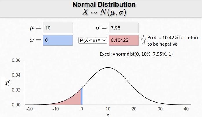

https://homepage.divms.uiowa.edu/~mbognar/applets/normal.html
Chapter 9 Stock
Return Evaluation
For class discussion:
· What is the dividend growth model, and
why do we use dividends to estimate a company's true value?
· Can we reliably predict future dividend
payments?
· Why do we require returns estimated
based on risk factors to determine stock prices?
Refer to the following table for WMT’s
dividend history
https://www.nasdaq.com/market-activity/stocks/wmt/dividend-history
WMT Dividend History
·
EX-DIVIDEND DATE 12/07/2023
·
DIVIDEND YIELD 1.31%
·
ANNUAL DIVIDEND $2.28
·
P/E RATIO 30.26
|
Ex/EFF Date |
Type |
Cash Amount |
Declaration
Date |
Record Date |
Payment Date |
|
05/09/2024 |
Cash |
$0.2075 |
02/20/2024 |
05/10/2024 |
05/28/2024 |
|
03/14/2024 |
Cash |
$0.2075 |
02/20/2024 |
03/15/2024 |
04/01/2024 |
|
12/07/2023 |
Cash |
$0.57 |
02/21/2023 |
12/08/2023 |
01/02/2024 |
|
08/10/2023 |
Cash |
$0.57 |
02/17/2023 |
08/11/2023 |
09/05/2023 |
|
05/04/2023 |
Cash |
$0.57 |
02/21/2023 |
05/05/2023 |
05/30/2023 |
|
03/16/2023 |
Cash |
$0.57 |
02/21/2023 |
03/17/2023 |
04/03/2023 |
|
12/08/2022 |
Cash |
$0.56 |
02/17/2022 |
12/09/2022 |
01/03/2023 |
|
08/11/2022 |
Cash |
$0.56 |
02/17/2022 |
08/12/2022 |
09/06/2022 |
|
05/05/2022 |
Cash |
$0.56 |
02/17/2022 |
05/06/2022 |
05/31/2022 |
|
03/17/2022 |
Cash |
$0.56 |
02/17/2022 |
03/18/2022 |
04/04/2022 |
|
12/09/2021 |
Cash |
$0.55 |
02/18/2021 |
12/10/2021 |
01/03/2022 |
|
08/12/2021 |
Cash |
$0.55 |
02/18/2021 |
08/13/2021 |
09/07/2021 |
|
05/06/2021 |
Cash |
$0.55 |
02/18/2021 |
05/07/2021 |
06/01/2021 |
|
03/18/2021 |
Cash |
$0.55 |
02/18/2021 |
03/19/2021 |
04/05/2021 |
|
12/10/2020 |
Cash |
$0.54 |
02/18/2020 |
12/11/2020 |
01/04/2021 |
|
08/13/2020 |
Cash |
$0.54 |
02/18/2020 |
08/14/2020 |
09/08/2020 |
|
05/07/2020 |
Cash |
$0.54 |
02/18/2020 |
05/08/2020 |
06/01/2020 |
|
03/19/2020 |
Cash |
$0.54 |
02/18/2020 |
03/20/2020 |
04/06/2020 |
|
12/05/2019 |
Cash |
$0.53 |
02/19/2019 |
12/06/2019 |
01/02/2020 |
|
08/08/2019 |
Cash |
$0.53 |
02/19/2019 |
08/09/2019 |
09/03/2019 |
|
05/09/2019 |
Cash |
$0.53 |
02/19/2019 |
05/10/2019 |
06/03/2019 |
|
03/14/2019 |
Cash |
$0.53 |
02/19/2019 |
03/15/2019 |
04/01/2019 |
|
12/06/2018 |
Cash |
$0.52 |
02/21/2018 |
12/07/2018 |
01/02/2019 |
|
08/09/2018 |
Cash |
$0.52 |
02/21/2018 |
08/10/2018 |
09/04/2018 |
|
05/10/2018 |
Cash |
$0.52 |
02/20/2018 |
05/11/2018 |
06/04/2018 |
|
03/08/2018 |
Cash |
$0.52 |
02/20/2018 |
03/09/2018 |
04/02/2018 |
|
12/07/2017 |
Cash |
$0.51 |
02/21/2017 |
12/08/2017 |
01/02/2018 |
|
08/09/2017 |
Cash |
$0.51 |
02/21/2017 |
08/11/2017 |
09/05/2017 |
|
05/10/2017 |
Cash |
$0.51 |
02/21/2017 |
05/12/2017 |
06/05/2017 |
|
03/08/2017 |
Cash |
$0.51 |
02/21/2017 |
03/10/2017 |
04/03/2017 |
|
12/07/2016 |
Cash |
$0.50 |
02/18/2016 |
12/09/2016 |
01/03/2017 |
|
08/10/2016 |
Cash |
$0.50 |
02/18/2016 |
08/12/2016 |
09/06/2016 |
|
05/11/2016 |
Cash |
$0.50 |
02/18/2016 |
05/13/2016 |
06/06/2016 |
|
03/09/2016 |
Cash |
$0.50 |
02/18/2016 |
03/11/2016 |
04/04/2016 |
|
12/02/2015 |
Cash |
$0.49 |
02/19/2015 |
12/04/2015 |
01/04/2016 |
|
08/05/2015 |
Cash |
$0.49 |
02/19/2015 |
08/07/2015 |
09/08/2015 |
|
05/06/2015 |
Cash |
$0.49 |
02/19/2015 |
05/08/2015 |
06/01/2015 |
|
03/11/2015 |
Cash |
$0.49 |
02/19/2015 |
03/13/2015 |
04/06/2015 |
|
12/03/2014 |
Cash |
$0.48 |
02/20/2014 |
12/05/2014 |
01/05/2015 |
|
08/06/2014 |
Cash |
$0.48 |
02/20/2014 |
08/08/2014 |
09/03/2014 |
|
05/07/2014 |
Cash |
$0.48 |
02/20/2014 |
05/09/2014 |
06/02/2014 |
|
03/07/2014 |
Cash |
$0.48 |
02/20/2014 |
03/11/2014 |
04/01/2014 |
|
12/04/2013 |
Cash |
$0.47 |
02/21/2013 |
12/06/2013 |
01/02/2014 |
|
08/07/2013 |
Cash |
$0.47 |
02/21/2013 |
08/09/2013 |
09/03/2013 |
|
05/08/2013 |
Cash |
$0.47 |
02/21/2013 |
05/10/2013 |
06/03/2013 |
|
03/08/2013 |
Cash |
$0.47 |
02/21/2013 |
03/12/2013 |
04/01/2013 |
Can
you write down the math equation now?
WMT
stock price = ?
Can
you calculate now? It is hard right because we assume dividend payment goes
to infinity. How can we simplify the calculation?
We
can assume that dividend grows at certain rate, just as the table on the
right shows.
Discount
rate is r (based on Beta and CAPM learned in chapter8)
Dividend growth model:

Refer to http://www.calculatinginvestor.com/2011/05/18/gordon-growth-model/
· Now let’s apply this
Dividend growth model in problem solving.
Dividend
  Growth Model Calculator
(www.jufinance.com/stock
)
Equations
Po = D1/(r-g) = Do*(1+g)/(r-g),
Where D1= next dividend; Do = just paid
dividend; r=stock return; g= dividend growth rate; Po= current market
price
Dividend Yield = D1/Po = Do*(1+g) / Po
Capital gain yield = (P1/Po) -1 = g
Total return = dividend yield + capital gain yield = D1/Po + g
Non-constant dividend growth model (www.jufinance.com/dcf)
Equations
Pn = Dn+1/(r-g) = Dn*(1+g)/(r-g), since
year n, dividends start to grow at a constant rate.
Where Dn+1= next dividend in year
n+1;
Do = just paid dividend in year n;
r=stock return; g= dividend growth rate;
Pn= current market price in year n;
Po = npv(r, D1, D2, …, Dn+Pn)
Or,
Po = D1/(1+r) + D2/(1+r)^2 + … +
(Dn+Pn)/(1+r)^n
In class exercise
2.
You expect AAA Corporation to
generate the following free cash flows over the next five years:
|
Year |
1 |
2 |
3 |
4 |
5 |
|
FCF
($ millions) |
75 |
84 |
96 |
111 |
120 |
Since
year 6, you estimate that AAA's free cash flows will grow at 6% per year.
WACC of AAA = 15%
· Calculate
the enterprise value for DM Corporation.
· Assume
that AAA has $500 million debt and 14 million shares outstanding, calculate
its stock price.
Answer:
Enterprise
value = npv(15%, 75, 84, 96, 111, 120+120*(1+6%)/(15%-6%)) = 1017.66
(hint: terminal
value in year 5 = 120*(1+6%)/(15%-6%))
(or, equity
value = 75/(1+15%) + 84/(1+15%)^2 + 96/(1+15%)^3 + 111/(1+15%)^4 +
(120+120*(1+6%)/(15%-6%))/(1+15%)^5
Equity
value = 1017.66-500 = 517.66
Stock
price = 517.66/14=37
NPV Excel
syntax
Syntax
NPV(rate,value1,value2,
...)
Rate
is the rate of discount over the length of one period.
Value1, value2,
...
are 1 to 29 arguments representing the payments and income.
· Value1, value2,
... must be equally spaced in time and occur at the end of
each period. NPV uses the order of value1, value2,
... to interpret the order of cash flows. Be sure to enter your payment
and income values in the correct sequence.
2. AAA’s divided yield = 2.5%, equity cost =
10%, and its dividends will grow at a constant rate of g. How much is g?
A) 2.5%
B) 5.0%
C) 10.0%
D) 7.5%
Answer:
Dividend yield + capital gain
yield = total return = 10%, and g= capital yield = dividend growth rate, so g
= 10% - 2.5% = 7.5%
3. AAA pays no dividend
currently. However, you expect it pay an annual dividend of $0.56/share 2
years from now with a growth rate of 4% per year thereafter. Its equity cost
= 12%, then its stock price=?
A) $4.67
B) $5.00
C) $6.25
D) $7.00
Answer:
Stock price = Po = npv(12%, 0,
0.56 + 0.56*(1+4%)/(12%-4%)) = 6.25
Or, Po = 0.56/(1+12%)^2 + 0.56*(1+4%)/(12%-4%)
/(1+12%)^2 = 6.25
4. AAA expects to have earnings
of $2.50 per share this coming year. It will retain all of the earnings for
the next year. For the following 3 years, it will retain 50% of its earnings. It will retain
25% of its earnings after that. Each year, retained earnings will be used in
new projects with a return of 20% per year as expected. The rest of retained
earnings will paid to shareholders as dividends. Its equity cost = 10%. Its
stock price=?
A) $40.80
B) $44.70
C) $59.80
D) $63.50
|
Year |
EPS |
Retained Earnings |
Growth in Earnings
(.20 × R.E.) |
Dividends |
|
1 |
$2.50 |
$2.50 |
|
|
|
2 |
|
|
|
|
|
3 |
|
|
|
|
|
4 |
|
|
|
|
|
5 |
|
|
|
|
Hint: after year 5, the growth rate =0.2/3.99 = 5%
Answer:
|
Year |
EPS |
Retained Earnings |
Growth in Earnings
(.20 × R.E.) |
Dividends |
|
1 |
$2.50 |
$2.50 |
0.5 |
0 |
|
2 |
3 |
1.5 |
0.3 |
1.5 |
|
3 |
3.3 |
1.65 |
0.33 |
1.65 |
|
4 |
3.63 |
1.82 |
0.36 |
1.82 |
|
5 |
3.99 |
1 |
0.2 |
3 |
after year 5, the growth rate
=0.2/3.99 = 5% = growth in earnings / EPS
So price at year 4 = 3/(10%-5%)
=60
So current stock price =
1.5/(1+10%)^2 + 1.65/(1+10%)^3 + 1.82/(1+10%)^4 + 60/(1+10%)^4 = 44.70
Or price = npv(10%, 0, 1.5, 1.65,
1.82+60)
Case Study chapter 9 (due with the Second Midterm
Exam)
Class Video 2-27-2024 (Thanks, Levi)
Stock screening tools
·
Reuters stock screener to help select stocks
http://stockscreener.us.reuters.com/Stock/US/
·
FINVIZ.com
http://finviz.com/screener.ashx
·
WSJ stock screen
http://online.wsj.com/public/quotes/stock_screener.html
·
Simply the Web's Best Financial Charts
You can find analyst rating
from MSN money
For instance,
ANALYSTS RATINGS
Zacks average brokerage recommendation is Moderate
Buy
|
RECOMMENDATIONS |
CURRENT |
1
MONTH AGO |
2
MONTHS AGO |
3
MONTHS AGO |
|
Strong
Buy |
26 |
26 |
25 |
24 |
|
Moderate
Buy |
4 |
4 |
4 |
4 |
|
Hold |
8 |
8 |
8 |
9 |
|
Moderate
Sell |
0 |
0 |
0 |
0 |
|
Strong
Sell |
0 |
0 |
0 |
0 |
|
Mean
Rec. |
1.51 |
1.51 |
1.53 |
1.58 |
Summary of stock screening rules from class discussion
PEG<1
PE<15 (? FB’s PE>100?)
Growth rate<20
ROE>10%
Analyst ranking: strong buy only
Zacks average =1 (from Ranking stocks
using PEG ratio)
current price>5
How to
pick stocks
Capital Asset Pricing Model
(CAPM)Explained
http://www.youtube.com/watch?v=JApBhv3VLTo
Ranking stocks using PEG ratio
http://www.youtube.com/watch?v=bekW_hTehNU
P/E Ratio Summary by industry (FYI)
(http://pages.stern.nyu.edu/~adamodar/New_Home_Page/datafile/pedata.html
|
Industry Name |
#of firms |
Current PE |
Expected growth - next 5 years |
PEG Ratio |
|
Advertising |
40 |
42.07 |
7.24% |
2.19 |
|
Aerospace/Defense |
87 |
45.24 |
11.46% |
2.08 |
|
Air Transport |
17 |
12.40 |
6.46% |
2.00 |
|
Apparel |
51 |
19.94 |
11.32% |
2.33 |
|
Auto & Truck |
18 |
15.03 |
18.35% |
0.80 |
|
Auto Parts |
62 |
23.32 |
12.64% |
1.17 |
|
Bank (Money Center) |
11 |
17.09 |
7.54% |
1.86 |
|
Banks (Regional) |
612 |
33.24 |
9.43% |
1.87 |
|
Beverage (Alcoholic) |
28 |
31.31 |
20.06% |
0.95 |
|
Beverage (Soft) |
35 |
28.28 |
10.77% |
2.99 |
|
Broadcasting |
27 |
31.34 |
7.59% |
2.58 |
|
Brokerage & Investment Banking |
42 |
31.77 |
11.70% |
1.39 |
|
Building Materials |
39 |
28.83 |
14.98% |
1.58 |
|
Business & Consumer Services |
169 |
59.52 |
12.94% |
2.01 |
|
Cable TV |
14 |
25.74 |
10.25% |
2.51 |
|
Chemical (Basic) |
38 |
28.39 |
14.14% |
1.38 |
|
Chemical (Diversified) |
7 |
281.02 |
18.82% |
2.28 |
|
Chemical (Specialty) |
99 |
145.32 |
12.34% |
2.04 |
|
Coal & Related Energy |
30 |
13.36 |
NA |
NA |
|
Computer Services |
111 |
48.66 |
12.36% |
1.37 |
|
Computers/Peripherals |
58 |
26.11 |
15.79% |
1.14 |
|
Construction Supplies |
49 |
35.67 |
15.00% |
2.21 |
|
Diversified |
24 |
38.63 |
12.48% |
1.96 |
|
Drugs (Biotechnology) |
459 |
127.65 |
27.31% |
0.65 |
|
Drugs (Pharmaceutical) |
185 |
46.35 |
20.47% |
1.32 |
|
Education |
34 |
132.99 |
11.91% |
2.35 |
|
Electrical Equipment |
118 |
29.63 |
15.09% |
1.75 |
|
Electronics (Consumer & Office) |
24 |
35.28 |
12.77% |
4.86 |
|
Electronics (General) |
167 |
56.36 |
17.82% |
1.42 |
|
Engineering/Construction |
49 |
28.75 |
12.30% |
1.92 |
|
Entertainment |
90 |
312.73 |
11.54% |
1.56 |
|
Environmental & Waste Services |
87 |
73.67 |
12.83% |
2.43 |
|
Farming/Agriculture |
34 |
22.90 |
15.33% |
1.42 |
|
Financial Svcs. (Non-bank & Insurance) |
264 |
41.45 |
11.62% |
0.88 |
|
Food Processing |
87 |
36.08 |
9.46% |
2.55 |
|
Food Wholesalers |
15 |
50.79 |
8.70% |
3.03 |
|
Furn/Home Furnishings |
31 |
17.82 |
13.40% |
1.43 |
|
Green & Renewable Energy |
22 |
89.05 |
11.05% |
2.91 |
|
Healthcare Products |
251 |
161.11 |
16.55% |
2.27 |
|
Healthcare Support Services |
115 |
38.56 |
14.52% |
1.37 |
|
Heathcare Information and Technology |
112 |
174.42 |
15.21% |
2.52 |
|
Homebuilding |
32 |
883.19 |
17.58% |
0.99 |
|
Hospitals/Healthcare Facilities |
35 |
58.93 |
6.50% |
2.09 |
|
Hotel/Gaming |
70 |
34.20 |
13.18% |
1.90 |
|
Household Products |
131 |
46.52 |
11.60% |
1.61 |
|
Information Services |
61 |
60.11 |
14.92% |
2.42 |
|
Insurance (General) |
21 |
34.97 |
10.46% |
2.11 |
|
Insurance (Life) |
25 |
152.83 |
7.82% |
1.52 |
|
Insurance (Prop/Cas.) |
50 |
120.04 |
11.56% |
1.64 |
|
Investments & Asset Management |
165 |
99.35 |
13.11% |
1.31 |
|
Machinery |
126 |
47.35 |
14.03% |
1.82 |
|
Metals & Mining |
102 |
28.08 |
30.62% |
0.92 |
|
Office Equipment & Services |
24 |
18.92 |
12.25% |
1.72 |
|
Oil/Gas (Integrated) |
5 |
45.20 |
25.77% |
1.26 |
|
Oil/Gas (Production and Exploration) |
311 |
25.17 |
1.81% |
7.33 |
|
Oil/Gas Distribution |
16 |
313.75 |
10.00% |
3.77 |
|
Oilfield Svcs/Equip. |
130 |
87.54 |
40.24% |
0.90 |
|
Packaging & Container |
25 |
51.42 |
9.31% |
2.31 |
|
Paper/Forest Products |
21 |
40.11 |
9.62% |
2.09 |
|
Power |
61 |
25.25 |
5.41% |
2.07 |
|
Precious Metals |
111 |
29.92 |
24.26% |
2.47 |
|
Publishing & Newspapers |
41 |
53.87 |
7.90% |
2.75 |
|
R.E.I.T. |
244 |
58.88 |
6.81% |
3.65 |
|
Real Estate (Development) |
20 |
20.24 |
NA |
NA |
|
Real Estate (General/Diversified) |
10 |
216.85 |
NA |
NA |
|
Real Estate (Operations & Services) |
60 |
486.19 |
13.63% |
1.39 |
|
Recreation |
70 |
27.16 |
12.23% |
1.90 |
|
Reinsurance |
3 |
11.75 |
8.75% |
2.27 |
|
Restaurant/Dining |
81 |
37.50 |
15.04% |
1.70 |
|
Retail (Automotive) |
25 |
14.30 |
16.63% |
0.96 |
|
Retail (Building Supply) |
8 |
46.86 |
20.46% |
1.21 |
|
Retail (Distributors) |
92 |
120.38 |
15.04% |
1.45 |
|
Retail (General) |
18 |
96.81 |
7.88% |
2.93 |
|
Retail (Grocery and Food) |
14 |
28.23 |
7.90% |
1.75 |
|
Retail (Online) |
61 |
73.27 |
20.77% |
3.70 |
|
Retail (Special Lines) |
106 |
43.48 |
11.59% |
1.52 |
|
Rubber& Tires |
4 |
13.28 |
9.50% |
0.85 |
|
Semiconductor |
72 |
49.82 |
15.68% |
1.30 |
|
Semiconductor Equip |
45 |
37.81 |
16.67% |
0.97 |
|
Shipbuilding & Marine |
9 |
18.23 |
13.50% |
1.96 |
|
Shoe |
11 |
95.38 |
12.39% |
2.17 |
|
Software (Entertainment) |
13 |
67.28 |
14.94% |
2.56 |
|
Software (Internet) |
305 |
205.58 |
27.74% |
1.03 |
|
Software (System & Application) |
255 |
209.66 |
17.06% |
1.90 |
|
Steel |
37 |
28.91 |
12.22% |
1.53 |
|
Telecom (Wireless) |
18 |
64.32 |
10.83% |
2.27 |
|
Telecom. Equipment |
104 |
114.62 |
14.42% |
1.36 |
|
Telecom. Services |
66 |
61.28 |
5.99% |
2.77 |
|
Tobacco |
24 |
29.52 |
10.33% |
1.30 |
|
Transportation |
18 |
82.37 |
15.49% |
1.74 |
|
Transportation (Railroads) |
8 |
27.22 |
10.56% |
2.26 |
|
Trucking |
30 |
29.95 |
21.01% |
1.54 |
|
Utility (General) |
18 |
27.54 |
5.50% |
4.30 |
|
Utility (Water) |
23 |
141.22 |
8.99% |
3.66 |
|
Total Market |
7247 |
71.28 |
13.60% |
1.58 |
|
Total Market (without financials) |
6057 |
75.42 |
14.19% |
1.64 |
Details about how
  to derive the model mathematically (FYI)
The Gordon growth model is a simple
discounted cash flow (DCF) model which can be used to value a stock, mutual
fund, or even the entire stock market. The model is named after Myron
Gordon who first published the model in 1959.
The Gordon model assumes that a
financial security pays a periodic dividend (D) which
grows at a constant rate (g). These growing dividend payments are
assumed to continue forever. The future dividend payments are discounted at
the required rate of return (r) to find the price (P) for the stock
or fund.
Under these simple assumptions, the
price of the security is given by this equation:
![]()
In this equation, I’ve used
the “0” subscript on the price (P) and the “1” subscript
on the dividend (D) to indicate that the price is calculated at time zero and
the dividend is the expected dividend at the end of period one. However, the
equation is commonly written with these subscripts omitted.
Obviously, the assumptions built
into this model are overly simplistic for many real-world valuation
problems. Many companies pay no dividends, and, for those that do,
we may expect changing payout ratios or growth rates as the
business matures.
Despite these limitations, I believe spending some
time experimenting with the Gordon model can help develop intuition
about the relationship between valuation and return.
Deriving the Gordon Growth Model
Equation
The Gordon growth model calculates the
present value of the security by summing an infinite series of discounted
dividend payments which follows the pattern shown here:
![]()
Multiplying both sides of the previous
equation by (1+g)/(1+r) gives:
![]()
We can then subtract the second equation
from the first equation to get:
![]()
Rearranging and simplifying:
![]()
![]()
Finally, we can simplify further to get the Gordon growth model
equation
Chapter 10 WACC
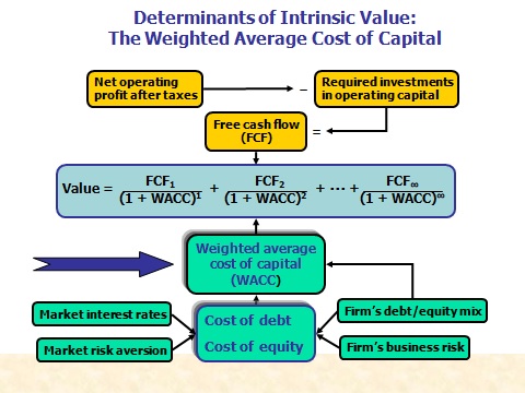
One option (if beta is given)

Another option (if dividend is given):
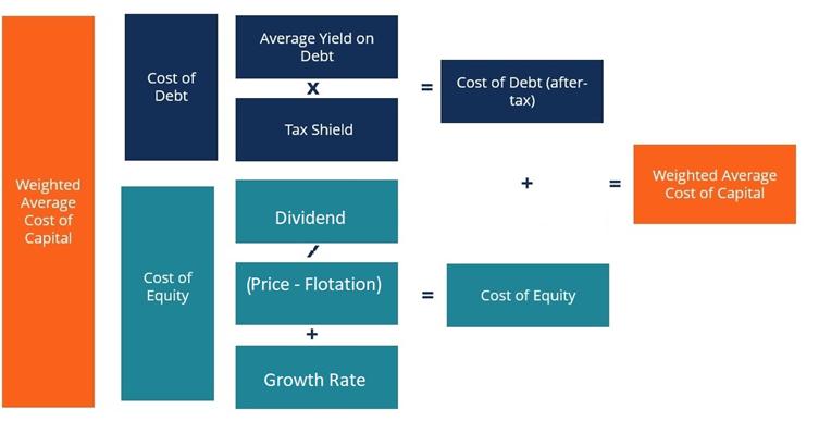
WACC Formula

WACC calculator (annual coupon bond)
(www.jufinance.com/wacc)
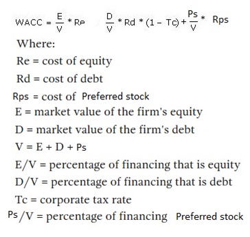
WACC calculator (semi-annual coupon bond)
WACC Calculator help videos FYI
Summary of Equations
Discount rate to figure out the value of projects is called WACC
(weighted average cost of capital)
WACC = weight of debt * cost of debt + weight
of equity *( cost of equity)
·
Wd= total debt / Total capital
= total borrowed / total capital
·
We= total equity/ Total capital
·
Cost of debt = rate(nper, coupon, -(price – flotation costs), 1000)*(1-tax rate)
·
Cost of Equity = D1/(Po – Flotation Cost) + g
·
D1: Next period dividend; Po: Current stock price; g: dividend
growth rate
·
Note: flotation costs = flotation percentage * price
·
Or if beta is given, use CAPM model
1.
Cost of equity = risk free rate + beta *(market return – risk
free rate)
2.
Cost of equity = risk free rate + beta * market risk premium
(FYI: Hertz Global Holdings Inc (NYSE:HTZ) WACC
%:5.21% As of 2/21/2024
As of today (2024-02-21),
Hertz Global Holdings's weighted average cost of capital is 5.21%%.
Hertz Global Holdings's ROIC % is 7.05% (calculated
using TTM income statement data). Hertz Global Holdings generates higher
returns on investment than it costs the company to raise the capital needed
for that investment. It is earning excess returns. A firm that expects to
continue generating positive excess returns on new investments in the future
will see its value increase as growth increases.
*Note: The
beta of this company cannot be obtained because it has a price history
shorter than 3 years. It will thus be set to 1 as default to calculate WACC. https://www.gurufocus.com/term/wacc/HTZ/WACC/Hertz+Global+Holdings+Inc
Hertz
Global Holdings WACC % Calculation
The weighted
average cost of capital (WACC) is the rate that a company is expected to pay
on average to all its security holders to finance its assets. The WACC is
commonly referred to as the firm's cost of capital. Generally speaking, a
company's assets are financed by debt and equity. WACC is the average of the
costs of these sources of financing, each of which is weighted by its
respective use in the given situation. By taking a weighted average, we can
see how much interest the company has to pay for every dollar it finances.
|
WACC |
= |
E |
/ |
(E
+ D) |
* |
Cost
of Equity |
+ |
D |
/ |
(E
+ D) |
* |
Cost
of Debt |
* |
(1
- Tax Rate) |
1. Weights:
Generally speaking, a company's assets are financed by debt and equity. We
need to calculate the weight of equity and the weight of debt.
The market value of equity (E) is also called "Market Cap".
As of today, Hertz Global Holdings's market capitalization (E) is $2219.504
Mil.
The market value of debt is typically difficult to calculate, therefore,
GuruFocus uses book value of debt (D) to do the calculation. It is simplified
by adding the latest one-year quarterly average Short-Term
Debt & Capital Lease Obligation and Long-Term Debt
& Capital Lease Obligation together. As of Dec. 2023,
Hertz Global Holdings's latest one-year quarterly average Book Value of Debt
(D) is $17397.6 Mil.
a) weight of equity = E / (E + D) = 2219.504 / (2219.504 + 17397.6) = 0.1131
b) weight of debt = D / (E + D) = 17397.6 / (2219.504 + 17397.6) = 0.8869
2. Cost of Equity:
GuruFocus uses Capital Asset Pricing Model (CAPM) to calculate the required
rate of return. The formula is:
Cost of Equity = Risk-Free Rate of Return + Beta of Asset * (Expected Return
of the Market - Risk-Free Rate of Return)
a) GuruFocus uses 10-Year Treasury Constant Maturity Rate as the risk-free
rate. It is updated daily. The current risk-free rate is 4.307%. Please go
to Economic
Indicators page for more information. Please note that we use
the 10-Year Treasury Constant Maturity Rate of the country/region where the
company is headquartered. If the data for that country/region is not
available, then we will use the 10-Year Treasury Constant Maturity Rate of
the United States as default.
b) Beta is the sensitivity of the expected excess asset returns to the
expected excess market returns. Hertz Global Holdings's beta cannot be
obtained because it has a price history shorter than 3 years. It will thus be
set to 1 as default to calculate WACC.
c) (Expected Return of the Market - Risk-Free Rate of Return) is also called
market premium. GuruFocus requires market premium to be 6%.
Cost of Equity = 4.307% + 1 * 6% = 10.307%
3. Cost of Debt:
GuruFocus uses latest TTM Interest
Expense divided by the latest one-year quarterly average debt
to get the simplified cost of debt.
As of Dec. 2023, Hertz Global Holdings's interest expense (positive number)
was $793 Mil. Its total Book Value of Debt (D) is $17397.6 Mil.
Cost of Debt = 793 / 17397.6 = 4.5581%.
4. Multiply by one minus TTM Tax Rate:
GuruFocus uses the most recent TTM Tax Expense divided
by the most recent TTM Pre-Tax Income to
calculate the tax rate. The calculated TTM tax rate is limited to between 0%
and 100%. If the calculated tax rate is higher than 100%, it is set to 100%.
If the calculated tax rate is less than 0%, it is set to 0%.
The latest calculated TTM Tax Rate = -330 / 286 = -115.38%, which is less
than 0%. Therefore it's set to 0%.
Hertz Global
Holdings's Weighted Average Cost Of Capital (WACC) for Today is
calculated as:
|
WACC |
= |
E
/ (E + D) |
* |
Cost
of Equity |
+ |
D
/ (E + D) |
* |
Cost
of Debt |
* |
(1
- Tax Rate) |
|
= |
0.1131 |
* |
10.307% |
+ |
0.8869 |
* |
4.5581% |
* |
(1
- 0%) |
|
|
= |
5.21% |
HERTZ WACC in 2017
Excel file is here. Thanks to Chris, Brian and Hanna,
the CFA competition team of 2017.
In Class Exercise (https://www.jufinance.com/fin435_24s/wacc_in_class_exercise.html)
1.
IBM financed 10m via debt coupon 5%, 10 year, price is $950 and
flotation is 7% of the price, tax 40%.
IBM financed 20m via equity. D1=$5. Po=50, g
is 5%. Flotation cost =0. So WACC?
Answer:
·
Kd
= rate(10, 5%*1000, -(950-950*7%),
1000)*(1-40%) = 3.98%------ after tax cost of debt
·
Ke
= 5/(50 – 0) + 5% =15% -------- cost
of equity
·
WACC
= Wd*Kd +We*Ke = (1/3)*3.98% + (2/3)*15% =11.33%
2.
Firm
AAA sold a noncallable bond now has 20 years to maturity. 9.25%
annual coupon rate, paid semiannually, sells at a price = $1,075, par =
$1,000. Tax rate = 40%, calculate after tax cost of debt (5.08%)
Answer:
·
after
tax cost of debt = rate(nper, coupon, -(price-flotation), 1000)*(1-tax rate)
·
After
tax of debt = rate(20*2, 9.25%*1000/2, -(1075-0), 1000)*(1-40%)=5.08%
3. Firm AAA’s
equity condition is as follows. D1 = $1.25; P0 =
$27.50; g = 5.00%; and Flotation = 6.00% of price. Calculate cost
of equity (9.84%)
Answer:
·
Cost
of equity = D1/(Po-flotation) + g= 1.25/(27.5-6%*27.5) + 5% = 9.84%
4. Continue from above. Firm
AAA raised 10m from the capital market. In it, 3m is from the debt market and
the rest from the equity market. Calculate WACC.
Answer:
·
WACC
= Wd*Kd +We*Ke =
·
WACC
= (3/10)*5.08% + (7/10)*9.84%
5. Common stock currently
sells =
$45.00 /
share; and earn $2.75 /share this year, payout
ratio is 70%, and its constant growth rate = 6.00%.
New stock can
be sold at the current price, a flotation cost =8%. How much would the cost
of new stock beyond
the cost of retained earnings?
Answer:
Expected EPS1 $2.75
Payout ratio 70%
Current stk price $45.00
g 6.00%
F 8.00%
D1 $1.925
rs = D1/P0 + g 10.28%
re = D1/(P0 ×
(1 − F)) + g 10.65%
Difference = re – rs 0.37%
6. (1) The firm's noncallable bonds mature in
20 years, an 8.00% annual coupon, a market price of $1,050.00. (2) tax rate = 40%.
(3) The risk-free rate=4.50%,
the market risk premium =
5.50%, stock’s
beta =1.20. (4) capital
structure consists of 35% debt and
65% common equity.
What is its WACC?
Answer:
Coupon rate 8.00%
Maturity 20
Bond price $1,050.00
Par value $1,000
Tax rate 40%
rRF 4.50%
RPM 5.50%
b 1.20
Weight debt 35%
Weight equity 65%
Bond
yield
7.51% (=rate(20,
8%*1000, -1050, 1000)
A-T
cost of debt 4.51% (=
rate(20, 8%*1000, -1050, 1000)*(1-40%)
Cost of equity, rs = rRF + b(RPM)
11.10% (=4.5% + 1.2*5.5%)
WACC = wd(rd)(1
– T) + wc(rs) = 8.79% (=35%*4.51% + 65% * 11.1%)
· WACC Case
study (due with the 2nd midterm exam)
·
Case Study In
Class Video (3/5/2024)
·
Critical Thinking
Challenge:
When comparing the WACC
for Apple from the two provided sources (as shown in the tables below), which
source do you consider to provide a more reliable WACC estimation?
Additionally, could you calculate the market value of equity based on the
WACC determined by each method?
·
https://www.gurufocus.com/term/wacc/AAPL/WACC-Percentage/Apple
·
https://valueinvesting.io/AAPL/valuation/wacc
Shares outstanding = 15.44B (https://ycharts.com/companies/AAPL/shares_outstanding)
FCF of 2023 = 106.9B (https://www.alphaspread.com/security/nasdaq/aapl/financials/cash-flow-statement/free-cash-flow)
For FCF growth rate, let's simplify the calculation by using a
7% discount rate.
Refer to https://www.stock-analysis-on.net/NASDAQ/Company/Apple-Inc/DCF/Present-Value-of-FCFF
for a more appropriate growth rate.
gurufocus.com:
|
Step
|
Calculation
|
Value |
|
Market Value of Equity
(E) |
$2,805,094.894
Billion |
- |
|
Book Value of Debt
(D) |
$109,826.6 Million
|
- |
|
Weight of Equity |
E/(E+D)
|
0.9623 |
|
Weight of Debt |
D/(E+D) |
0.0377 |
|
Risk-Free Rate |
4.30% |
- |
|
Beta |
1.21 |
- |
|
Expected Market
Premium |
6% |
- |
|
Cost of Equity |
( Risk-Free Rate + Beta * Expected Market
Premium ) |
11.56% |
|
Interest Expense |
$2,930 Million |
- |
|
Cost of Debt |
(Interest Expense)/(Book
Value of Debt) |
2.67% |
|
Tax Rate |
14.80% |
- |
|
WACC |
Weight of Equity * Cost of Equity + Weight
of Debt * Cost of Debt * (1 - Tax
Rate) ) |
11.21% |
Valueinvesting.io
|
Component
|
Low Range |
High Range |
Selected Value |
|
Long-term bond
rate |
3.90% |
4.40% |
- |
|
Equity market risk
premium |
4.60% |
5.60% |
- |
|
Adjusted beta |
0.8 |
0.95 |
- (????)
|
|
Additional risk
adjustments |
0.00% |
0.50% |
- |
|
Cost of equity |
7.60% |
10.20% |
8.90% |
|
Tax rate |
14.60% |
15.20% |
14.90% |
|
Debt/Equity ratio |
0.04 |
0.04 |
- |
|
Cost of debt |
4.00% |
4.60% |
4.30% |
|
After-tax WACC |
7.40% |
9.90% |
- |
|
Selected WACC |
|
|
8.70% |
|
|
|
|
|
|
|||
|
Unlevered beta |
0.71 |
0.94 |
|
|
Relevered beta |
0.73 |
0.97 |
|
|
Adjusted relevered beta |
0.82 |
0.98 |
|


Unlevered Beta (βu):
·
Definition: Unlevered beta represents the systematic risk of a
company's assets without taking into account the effects of financial
leverage (debt).
·
Calculation: It is calculated based on the company's business
risk and industry risk, excluding the influence of financial structure.
·
Use: Unlevered beta is commonly used in the context of valuing a
company's operations or core business, as it reflects the inherent riskiness
of the company's underlying business activities.
Relevered Beta (βL):
·
Definition: Relevered beta represents the systematic risk of a
company's equity after accounting for the effects of financial leverage
(debt).
·
Calculation: It is calculated by unlevering the beta (removing
the effects of financial leverage), adjusting it for the company's capital
structure (using the debt-to-equity ratio), and then relevering it to reflect
the company's actual financial structure.
·
Use: Relevered beta is often used in the context of determining
the required rate of return for a company's equity or estimating the
company's cost of equity capital, taking into account its specific financial
structure.
https://www.wallstreetprep.com/knowledge/beta-levered-unlevered/
Hint:
Compare the reliability of
Apple's Weighted Average Cost of Capital (WACC) between the two websites by
calculating the market value of equity based on each method using Apple's
Free Cash Flow (FCF) in 2023 and a growth rate of 5% with the Dividend Growth
Model approach. Then, you'll calculate the stock price using the equity value
and the number of outstanding shares.
Here's the step-by-step
process:
1)
Calculate Equity Value:
Based on each website's WACC,
you'll calculate the firm value using the FCF and growth rate, subtract the
book value of debt to get the equity value.
·
Calculate firm value using the formula:
Firm Value = FCF 2023 × (1 + growth rate)/
(WACC − growth rate)
·
Calculate equity value:
Equity Value = Firm Value − Book Value of Debt
2)
Calculate Stock Price: Divide the equity value by the number of
outstanding shares to get the stock price.
·
Calculate stock price:
Stock Price = Equity Value /
Number of Outstanding Shares
Once you have the equity
values from both methods, you'll compare the differences in the calculated
stock prices.
Hint:
Corporate Bond Data is available at FINRA.ORG: https://www.finra.org/finra-data/fixed-income/corp-and-agency
Muni Bond Data is available at EMMA: https://emma.msrb.org/
Treasury Securities Data is available at Treasury Direct: https://www.treasurydirect.gov/
FYI: WACC calculator https://fairness-finance.com/fairness-finance/finance/calculator/wacc.dhtml
Cost of Capital by Sector (US)
https://pages.stern.nyu.edu/~adamodar/New_Home_Page/datafile/wacc.html
|
Industry Name |
Number of Firms |
Beta |
Cost of Equity |
E/(D+E) |
Std Dev in Stock |
Cost of Debt |
Tax Rate |
After-tax Cost of Debt |
D/(D+E) |
Cost of Capital |
|
Advertising |
58 |
1.63 |
13.57% |
68.97% |
52.72% |
5.88% |
6.39% |
4.41% |
31.03% |
10.73% |
|
Aerospace/Defense |
77 |
1.41 |
12.28% |
79.33% |
37.56% |
5.50% |
8.60% |
4.13% |
20.67% |
10.59% |
|
Air
Transport |
21 |
1.42 |
12.29% |
34.92% |
37.73% |
5.50% |
10.47% |
4.13% |
65.08% |
6.98% |
|
Apparel |
39 |
1.32 |
11.75% |
65.98% |
38.51% |
5.50% |
12.04% |
4.13% |
34.02% |
9.15% |
|
Auto
& Truck |
31 |
1.54 |
13.03% |
66.58% |
52.61% |
5.88% |
3.00% |
4.41% |
33.42% |
10.15% |
|
Auto
Parts |
37 |
1.47 |
12.64% |
70.10% |
39.52% |
5.50% |
9.30% |
4.13% |
29.90% |
10.09% |
|
Bank
(Money Center) |
7 |
1.08 |
10.30% |
31.61% |
19.59% |
4.73% |
16.25% |
3.55% |
68.39% |
5.68% |
|
Banks
(Regional) |
557 |
0.5 |
6.88% |
60.75% |
16.76% |
4.73% |
18.84% |
3.55% |
39.25% |
5.57% |
|
Beverage
(Alcoholic) |
23 |
1.01 |
9.90% |
81.36% |
49.87% |
5.50% |
9.39% |
4.13% |
18.64% |
8.82% |
|
Beverage
(Soft) |
31 |
1.3 |
11.62% |
86.75% |
41.72% |
5.50% |
6.42% |
4.13% |
13.25% |
10.63% |
|
Broadcasting |
26 |
1.32 |
11.73% |
40.51% |
46.90% |
5.50% |
15.76% |
4.13% |
59.49% |
7.21% |
|
Brokerage
& Investment Banking |
30 |
1.2 |
11.04% |
33.21% |
28.00% |
5.50% |
15.32% |
4.13% |
66.79% |
6.42% |
|
Building
Materials |
45 |
1.28 |
11.47% |
77.56% |
29.19% |
5.50% |
16.71% |
4.13% |
22.44% |
9.82% |
|
Business
& Consumer Services |
164 |
1.17 |
10.84% |
78.45% |
45.78% |
5.50% |
9.43% |
4.13% |
21.55% |
9.39% |
|
Cable
TV |
10 |
1.26 |
11.34% |
48.25% |
25.41% |
5.50% |
21.95% |
4.13% |
51.75% |
7.60% |
|
Chemical
(Basic) |
38 |
1.25 |
11.29% |
67.43% |
46.58% |
5.50% |
9.83% |
4.13% |
32.57% |
8.95% |
|
Chemical
(Diversified) |
4 |
1.41 |
12.27% |
63.19% |
39.49% |
5.50% |
12.02% |
4.13% |
36.81% |
9.27% |
|
Chemical
(Specialty) |
76 |
1.28 |
11.47% |
78.49% |
42.32% |
5.50% |
10.75% |
4.13% |
21.51% |
9.89% |
|
Coal
& Related Energy |
19 |
1.45 |
12.51% |
82.16% |
61.96% |
5.88% |
2.28% |
4.41% |
17.84% |
11.06% |
|
Computer
Services |
80 |
1.17 |
10.84% |
75.44% |
47.78% |
5.50% |
6.47% |
4.13% |
24.56% |
9.19% |
|
Computers/Peripherals |
42 |
1.29 |
11.55% |
91.31% |
48.73% |
5.50% |
9.13% |
4.13% |
8.69% |
10.90% |
|
Construction
Supplies |
49 |
1.26 |
11.39% |
76.85% |
35.11% |
5.50% |
10.52% |
4.13% |
23.15% |
9.71% |
|
Diversified |
23 |
1.04 |
10.05% |
82.48% |
57.84% |
5.88% |
2.98% |
4.41% |
17.52% |
9.06% |
|
Drugs
(Biotechnology) |
598 |
1.24 |
11.26% |
86.71% |
58.41% |
5.88% |
0.94% |
4.41% |
13.29% |
10.35% |
|
Drugs
(Pharmaceutical) |
281 |
1.27 |
11.41% |
88.02% |
64.88% |
5.88% |
2.37% |
4.41% |
11.98% |
10.57% |
|
Education |
33 |
1.1 |
10.42% |
76.56% |
41.81% |
5.50% |
7.10% |
4.13% |
23.44% |
8.94% |
|
Electrical
Equipment |
110 |
1.59 |
13.32% |
81.62% |
58.55% |
5.88% |
4.47% |
4.41% |
18.38% |
11.68% |
|
Electronics
(Consumer & Office) |
16 |
1.54 |
13.02% |
85.87% |
39.56% |
5.50% |
3.98% |
4.13% |
14.13% |
11.76% |
|
Electronics
(General) |
138 |
1.2 |
11.02% |
84.16% |
44.94% |
5.50% |
6.29% |
4.13% |
15.84% |
9.92% |
|
Engineering/Construction |
43 |
1.2 |
10.99% |
75.99% |
35.17% |
5.50% |
13.30% |
4.13% |
24.01% |
9.34% |
|
Entertainment |
110 |
1.45 |
12.49% |
75.03% |
57.81% |
5.88% |
3.45% |
4.41% |
24.97% |
10.47% |
|
Environmental
& Waste Services |
62 |
1.02 |
9.91% |
79.66% |
48.09% |
5.50% |
5.42% |
4.13% |
20.34% |
8.73% |
|
Farming/Agriculture |
39 |
1.14 |
10.65% |
74.70% |
54.43% |
5.88% |
6.64% |
4.41% |
25.30% |
9.07% |
|
Financial
Svcs. (Non-bank & Insurance) |
223 |
0.89 |
9.14% |
9.05% |
27.15% |
5.50% |
14.61% |
4.13% |
90.95% |
4.58% |
|
Food
Processing |
92 |
0.92 |
9.33% |
77.60% |
34.23% |
5.50% |
7.74% |
4.13% |
22.40% |
8.16% |
|
Food
Wholesalers |
14 |
1.12 |
10.55% |
68.42% |
32.42% |
5.50% |
11.94% |
4.13% |
31.58% |
8.52% |
|
Furn/Home
Furnishings |
32 |
1.27 |
11.43% |
64.13% |
41.91% |
5.50% |
12.67% |
4.13% |
35.87% |
8.81% |
|
Green
& Renewable Energy |
19 |
1.6 |
13.39% |
45.23% |
67.60% |
7.01% |
6.73% |
5.26% |
54.77% |
8.93% |
|
Healthcare
Products |
254 |
1.16 |
10.78% |
88.81% |
50.94% |
5.88% |
3.70% |
4.41% |
11.19% |
10.07% |
|
Healthcare
Support Services |
131 |
1.16 |
10.77% |
80.90% |
47.79% |
5.50% |
6.74% |
4.13% |
19.10% |
9.50% |
|
Heathcare
Information and Technology |
138 |
1.47 |
12.62% |
87.56% |
53.87% |
5.88% |
4.30% |
4.41% |
12.44% |
11.60% |
|
Homebuilding |
32 |
1.5 |
12.80% |
75.57% |
33.33% |
5.50% |
17.81% |
4.13% |
24.43% |
10.68% |
|
Hospitals/Healthcare
Facilities |
34 |
1.17 |
10.85% |
53.41% |
51.19% |
5.88% |
9.56% |
4.41% |
46.59% |
7.85% |
|
Hotel/Gaming |
69 |
1.46 |
12.55% |
60.03% |
38.05% |
5.50% |
8.14% |
4.13% |
39.97% |
9.18% |
|
Household
Products |
127 |
1.16 |
10.74% |
86.56% |
56.83% |
5.88% |
6.73% |
4.41% |
13.44% |
9.89% |
|
Information
Services |
73 |
1.4 |
12.22% |
88.45% |
45.11% |
5.50% |
12.45% |
4.13% |
11.55% |
11.29% |
|
Insurance
(General) |
21 |
1.23 |
11.17% |
76.63% |
43.76% |
5.50% |
10.26% |
4.13% |
23.37% |
9.53% |
|
Insurance
(Life) |
27 |
0.94 |
9.46% |
51.97% |
28.89% |
5.50% |
11.41% |
4.13% |
48.03% |
6.90% |
|
Insurance
(Prop/Cas.) |
51 |
0.8 |
8.65% |
82.33% |
27.67% |
5.50% |
10.92% |
4.13% |
17.67% |
7.85% |
|
Investments
& Asset Management |
600 |
0.62 |
7.58% |
72.28% |
9.91% |
4.73% |
4.01% |
3.55% |
27.72% |
6.47% |
|
Machinery |
116 |
1.22 |
11.16% |
82.75% |
32.36% |
5.50% |
10.37% |
4.13% |
17.25% |
9.94% |
|
Metals
& Mining |
68 |
1.29 |
11.54% |
82.27% |
70.06% |
7.01% |
4.15% |
5.26% |
17.73% |
10.43% |
|
Office
Equipment & Services |
16 |
1.18 |
10.87% |
59.95% |
35.22% |
5.50% |
19.53% |
4.13% |
40.05% |
8.17% |
|
Oil/Gas
(Integrated) |
4 |
0.98 |
9.69% |
89.68% |
30.55% |
5.50% |
14.22% |
4.13% |
10.32% |
9.11% |
|
Oil/Gas
(Production and Exploration) |
174 |
1.26 |
11.35% |
83.28% |
56.98% |
5.88% |
4.60% |
4.41% |
16.72% |
10.19% |
|
Oil/Gas
Distribution |
23 |
0.99 |
9.77% |
58.34% |
33.55% |
5.50% |
6.90% |
4.13% |
41.66% |
7.42% |
|
Oilfield
Svcs/Equip. |
101 |
1.38 |
12.05% |
75.41% |
46.90% |
5.50% |
7.07% |
4.13% |
24.59% |
10.10% |
|
Packaging
& Container |
25 |
0.95 |
9.54% |
61.74% |
24.43% |
4.73% |
14.66% |
3.55% |
38.26% |
7.25% |
|
Paper/Forest
Products |
7 |
1.38 |
12.10% |
69.51% |
42.84% |
5.50% |
12.76% |
4.13% |
30.49% |
9.66% |
|
Power |
48 |
0.73 |
8.19% |
56.45% |
17.18% |
4.73% |
12.30% |
3.55% |
43.55% |
6.17% |
|
Precious
Metals |
74 |
1.23 |
11.21% |
85.97% |
72.54% |
7.01% |
2.87% |
5.26% |
14.03% |
10.37% |
|
Publishing
& Newspapers |
20 |
1.11 |
10.50% |
70.34% |
30.92% |
5.50% |
9.67% |
4.13% |
29.66% |
8.61% |
|
R.E.I.T. |
223 |
1.06 |
10.20% |
56.39% |
21.54% |
4.73% |
3.38% |
3.55% |
43.61% |
7.30% |
|
Real
Estate (Development) |
18 |
1.52 |
12.89% |
47.05% |
51.25% |
5.88% |
6.66% |
4.41% |
52.95% |
8.40% |
|
Real
Estate (General/Diversified) |
12 |
0.79 |
8.57% |
71.52% |
28.66% |
5.50% |
9.37% |
4.13% |
28.48% |
7.31% |
|
Real
Estate (Operations & Services) |
60 |
1.35 |
11.87% |
47.79% |
44.43% |
5.50% |
5.47% |
4.13% |
52.21% |
7.83% |
|
Recreation |
57 |
1.42 |
12.30% |
65.76% |
42.13% |
5.50% |
9.49% |
4.13% |
34.24% |
9.50% |
|
Reinsurance |
1 |
0.83 |
8.81% |
68.92% |
19.37% |
4.73% |
6.48% |
3.55% |
31.08% |
7.17% |
|
Restaurant/Dining |
70 |
1.41 |
12.26% |
76.47% |
41.15% |
5.50% |
8.54% |
4.13% |
23.53% |
10.34% |
|
Retail
(Automotive) |
30 |
1.52 |
12.91% |
63.50% |
35.71% |
5.50% |
15.84% |
4.13% |
36.50% |
9.70% |
|
Retail
(Building Supply) |
15 |
1.79 |
14.51% |
82.50% |
37.55% |
5.50% |
13.39% |
4.13% |
17.50% |
12.69% |
|
Retail
(Distributors) |
69 |
1.28 |
11.45% |
71.65% |
37.08% |
5.50% |
13.59% |
4.13% |
28.35% |
9.38% |
|
Retail
(General) |
15 |
1.36 |
11.98% |
83.35% |
31.53% |
5.50% |
21.26% |
4.13% |
16.65% |
10.67% |
|
Retail
(Grocery and Food) |
13 |
0.67 |
7.85% |
60.31% |
28.26% |
5.50% |
16.45% |
4.13% |
39.69% |
6.37% |
|
Retail
(Online) |
63 |
1.49 |
12.71% |
83.91% |
59.41% |
5.88% |
4.09% |
4.41% |
16.09% |
11.38% |
|
Retail
(Special Lines) |
78 |
1.48 |
12.64% |
71.86% |
38.59% |
5.50% |
15.02% |
4.13% |
28.14% |
10.25% |
|
Rubber&
Tires |
3 |
0.84 |
8.86% |
23.24% |
39.79% |
5.50% |
0.00% |
4.13% |
76.76% |
5.22% |
|
Semiconductor |
68 |
1.61 |
13.43% |
89.88% |
38.40% |
5.50% |
8.18% |
4.13% |
10.12% |
12.49% |
|
Semiconductor
Equip |
30 |
1.76 |
14.32% |
89.46% |
41.57% |
5.50% |
10.94% |
4.13% |
10.54% |
13.24% |
|
Shipbuilding
& Marine |
8 |
0.94 |
9.49% |
71.93% |
41.16% |
5.50% |
6.23% |
4.13% |
28.07% |
7.98% |
|
Shoe |
13 |
1.33 |
11.77% |
91.73% |
39.37% |
5.50% |
10.70% |
4.13% |
8.27% |
11.13% |
|
Software
(Entertainment) |
91 |
1.36 |
11.98% |
95.42% |
58.71% |
5.88% |
3.82% |
4.41% |
4.58% |
11.63% |
|
Software
(Internet) |
33 |
1.55 |
13.09% |
84.99% |
55.24% |
5.88% |
2.37% |
4.41% |
15.01% |
11.79% |
|
Software
(System & Application) |
390 |
1.47 |
12.61% |
91.44% |
52.11% |
5.88% |
3.40% |
4.41% |
8.56% |
11.91% |
|
Steel |
28 |
1.34 |
11.85% |
77.76% |
38.30% |
5.50% |
14.95% |
4.13% |
22.24% |
10.14% |
|
Telecom
(Wireless) |
16 |
1.03 |
10.00% |
60.55% |
51.92% |
5.88% |
3.83% |
4.41% |
39.45% |
7.80% |
|
Telecom.
Equipment |
79 |
1.23 |
11.20% |
89.54% |
41.35% |
5.50% |
4.06% |
4.13% |
10.46% |
10.46% |
|
Telecom.
Services |
49 |
0.88 |
9.12% |
45.93% |
55.37% |
5.88% |
6.54% |
4.41% |
54.07% |
6.57% |
|
Tobacco |
15 |
2 |
15.76% |
80.61% |
44.06% |
5.50% |
9.83% |
4.13% |
19.39% |
13.51% |
|
Transportation |
18 |
1.06 |
10.17% |
77.21% |
28.05% |
5.50% |
16.39% |
4.13% |
22.79% |
8.79% |
|
Transportation
(Railroads) |
4 |
1.11 |
10.46% |
78.46% |
16.34% |
4.73% |
16.57% |
3.55% |
21.54% |
8.97% |
|
Trucking |
35 |
1.55 |
13.06% |
69.49% |
41.17% |
5.50% |
14.79% |
4.13% |
30.51% |
10.33% |
|
Utility
(General) |
15 |
0.64 |
7.65% |
57.41% |
14.97% |
4.73% |
13.20% |
3.55% |
42.59% |
5.90% |
|
Utility
(Water) |
16 |
1.15 |
10.73% |
69.74% |
27.96% |
5.50% |
8.45% |
4.13% |
30.26% |
8.73% |
|
Total
Market |
7165 |
1.16 |
10.75% |
65.14% |
41.37% |
5.50% |
7.52% |
4.13% |
34.86% |
8.44% |
|
Total
Market (without financials) |
5649 |
1.29 |
11.56% |
79.11% |
47.98% |
5.50% |
6.38% |
4.13% |
20.89% |
10.01% |
*****
How much does Amazon worth in
2019?”
FYI: Amazon.com Inc. (AMZN) https://www.stock-analysis-on.net/NASDAQ/Company/Amazoncom-Inc/DCF/Present-Value-of-FCFF
Present
Value of Free Cash Flow to the Firm (FCFF)
In discounted cash flow (DCF) valuation techniques the value
of the stock is estimated based upon present value of some measure of cash
flow. Free cash flow to the firm (FCFF) is generally described as cash flows
after direct costs and before any payments to capital suppliers.
- Intrinsic Stock
Value (Valuation Summary)
- Weighted Average
Cost of Capital (WACC)
- FCFF Growth Rate
(g)
Intrinsic Stock Value (Valuation
Summary)
Amazon.com Inc., free cash flow to the firm (FCFF) forecast
|
Year |
Value |
FCFFt or Terminal value (TVt) |
Calculation |
Present value at 16.17% |
|
01 |
FCFF0 |
(4,286) |
||
|
1 |
FCFF1 |
– |
= (4,286) ×
(1 + 0.00%) |
– |
|
2 |
FCFF2 |
– |
= – ×
(1 + 0.00%) |
– |
|
3 |
FCFF3 |
– |
= – ×
(1 + 0.00%) |
– |
|
4 |
FCFF4 |
– |
= – ×
(1 + 0.00%) |
– |
|
5 |
FCFF5 |
– |
= – ×
(1 + 0.00%) |
– |
|
5 |
Terminal value (TV5) |
– |
= – ×
(1 + 0.00%) ÷ (16.17%
– 0.00%) |
– |
|
Intrinsic value of Amazon.com's capital |
– |
|||
|
Less: Debt (fair value) |
45,696 |
|||
|
Intrinsic value of Amazon.com's common
stock |
– |
|||
|
Intrinsic value of Amazon.com's common
stock (per share) |
$– |
|||
|
Current share price |
$1,642.81 |
|||
1
Weighted Average Cost of Capital
(WACC)
Amazon.com Inc., cost of capital
|
Value1 |
Weight |
Required rate of return2 |
Calculation |
|
|
Equity
(fair value) |
803,283 |
0.95 |
16.97% |
|
|
Debt
(fair value) |
45,696 |
0.05 |
2.10% |
= 2.99% × (1 – 29.84%) |
1 USD $ in millions
Equity (fair value) = No. shares of
common stock outstanding × Current share price
= 488,968,628 × $1,642.81 =
$803,282,551,764.68
Debt (fair value). See Details »
2 Required rate of return on equity
is estimated by using CAPM. See Details »
Required rate of return on
debt. See Details »
Required rate of return on debt is
after tax.
Estimated (average) effective
income tax rate
= (20.20% + 36.61%
+ 60.59% + 0.00%
+ 31.80%) ÷ 5 = 29.84%
WACC = 16.17%
FCFF Growth Rate (g)
FCFF growth rate (g) implied by PRAT model
Amazon.com Inc., PRAT model
|
Average |
Dec 31, 2017 |
Dec 31, 2016 |
Dec 31, 2015 |
Dec 31, 2014 |
Dec 31, 2013 |
||
|
Selected Financial Data
(USD $ in millions) |
|||||||
|
Interest expense |
848 |
484 |
459 |
210 |
141 |
||
|
Net income (loss) |
3,033 |
2,371 |
596 |
(241) |
274 |
||
|
Effective income tax rate (EITR)1 |
20.20% |
36.61% |
60.59% |
0.00% |
31.80% |
||
|
Interest expense, after tax2 |
677 |
307 |
181 |
210 |
96 |
||
|
Interest expense (after tax) and
dividends |
677 |
307 |
181 |
210 |
96 |
||
|
EBIT(1 – EITR)3 |
3,710 |
2,678 |
777 |
(31) |
370 |
||
|
Current portion of long-term debt |
100 |
1,056 |
238 |
1,520 |
753 |
||
|
Current portion of capital lease
obligation |
5,839 |
3,997 |
3,027 |
2,013 |
955 |
||
|
Current portion of finance lease
obligations |
282 |
144 |
99 |
67 |
28 |
||
|
Long-term debt, excluding current
portion |
24,743 |
7,694 |
8,235 |
8,265 |
3,191 |
||
|
Long-term capital lease obligations,
excluding current portion |
8,438 |
5,080 |
4,212 |
3,026 |
1,435 |
||
|
Long-term finance lease obligations,
excluding current portion |
4,745 |
2,439 |
1,736 |
1,198 |
555 |
||
|
Total stockholders' equity |
27,709 |
19,285 |
13,384 |
10,741 |
9,746 |
||
|
Total capital |
71,856 |
39,695 |
30,931 |
26,830 |
16,663 |
||
|
Ratios |
|||||||
|
Retention rate (RR)4 |
0.82 |
0.89 |
0.77 |
– |
0.74 |
||
|
Return on invested capital (ROIC)5 |
5.16% |
6.75% |
2.51% |
-0.12% |
2.22% |
||
|
Averages |
|||||||
|
RR |
0.80 |
||||||
|
ROIC |
3.31% |
||||||
|
Growth rate of FCFF (g)6 |
0.00% |
||||||
2017 Calculations
2 Interest expense, after tax = Interest expense × (1 –
EITR)
= 848 × (1 – 20.20%)
= 677
3 EBIT(1 – EITR) = Net income (loss) + Interest expense,
after tax
= 3,033 + 677 = 3,710
4 RR = [EBIT(1 – EITR) – Interest expense (after tax) and
dividends] ÷ EBIT(1 – EITR)
= [3,710 – 677]
÷ 3,710 = 0.82
5 ROIC = 100 × EBIT(1 – EITR) ÷ Total capital
= 100 × 3,710 ÷ 71,856 = 5.16%
6 g =
RR × ROIC
= 0.80 × 3.31%
= 0.00%
FCFF growth rate (g) forecast
Amazon.com Inc., H-model
|
Year |
Value |
gt |
|
1 |
g1 |
0.00% |
|
2 |
g2 |
0.00% |
|
3 |
g3 |
0.00% |
|
4 |
g4 |
0.00% |
|
5 and thereafter |
g5 |
0.00% |
where:
g1 is
implied by PRAT model
g5 is
implied by single-stage model
g2, g3 and g4 are
calculated using linear interpoltion between g1 and g5
Calculations
g2 = g1 +
(g5 – g1) × (2
– 1) ÷ (5 – 1)
= 0.00% + (0.00%
– 0.00%) × (2 – 1) ÷ (5 – 1) = 0.00%
g3 = g1 +
(g5 – g1) × (3
– 1) ÷ (5 – 1)
= 0.00% + (0.00%
– 0.00%) × (3 – 1) ÷ (5 – 1) = 0.00%
g4 = g1 +
(g5 – g1) × (4
– 1) ÷ (5 – 1)
= 0.00% + (0.00%
– 0.00%) × (4 – 1) ÷ (5 – 1) = 0.00%
Recommended websites for WACC
Hertz
·
https://valueinvesting.io/HTZGQ/valuation/wacc
https://www.gurufocus.com/term/wacc/HTZ/WACC/Hertz+Global+Holdings+Inc
Tesla
·
https://www.gurufocus.com/term/wacc/TSLA/WACC-Percentage/Tesla
·
https://valueinvesting.io/TSLA/valuation/wacc // cost of equity = long term bond rate +
premium
Wal-Mart
·
https://valueinvesting.io/WMT/valuation/wacc
Amazon
·
https://valueinvesting.io/AMZN/valuation/wacc
·
https://www.gurufocus.com/term/wacc/AMZN/WACC-Percentage/Amazon.com
Apple
·
https://www.gurufocus.com/term/wacc/AAPL/WACC-Percentage/Apple
·
https://valueinvesting.io/AAPL/valuation/wacc
Chapter 11: Capital Budgeting
1. NPV Excel syntax
Syntax
NPV(rate,value1,value2, ...)
Rate is the rate of discount over
the length of one period.
Value1, value2, ... are 1 to 29 arguments
representing the payments and income.
· Value1, value2, ... must be equally spaced in
time and occur at the end of each period. NPV uses the
order of value1, value2, ... to interpret the order of cash flows.
Be sure to enter your payment and income values in the correct sequence.
2. IRR Excel syntax
Syntax
IRR(values, guess)
Values is an array or a reference to cells
that contain numbers for which you want to calculate the internal rate of
return.
Guess is a number that you guess is
close to the result of IRR.
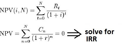
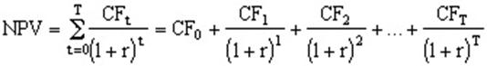
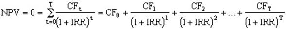
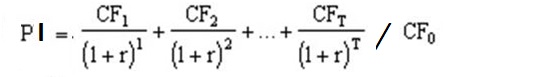
Or, PI =
NPV / CFo +1
Profitable
index (PI) =1 + NPV / absolute value of CFo
3. MIRR( values, finance_rate, reinvest_rate )
Where the function arguments are as follows:
|
Values |
- |
An array of values
(or a reference to a range of cells containing values) representing the
series of cash flows (investment and net income values) that occur at
regular periods. These must contain at least one negative value
(representing payment) and at least one positive value (representing
income). |
|
finance_rate |
- |
The interest rate paid on the money used in the cash
flows. |
|
reinvest_rate |
- |
The interest rate paid on the reinvested cash flows. |
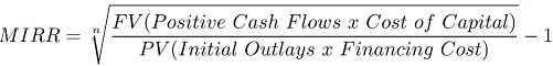
1)
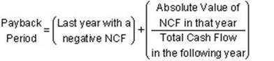
Summary:
|
Method |
Equation |
Ease of Use |
Potential Problems |
Popularity |
|
Net Present Value (NPV) |
NPV = ∑(Cash flows / (1 + Discount Rate)^n) - Initial
Investment |
Relatively easy to calculate in Excel using the NPV function |
Difficulty in estimating future cash flows accurately.
Sensitivity to changes in discount rate |
Very popular due to its focus on absolute value and
consideration of the time value of money |
|
Internal Rate of Return (IRR) |
NPV = 0, where NPV = ∑(Cash flows / (1 + IRR)^n) -
Initial Investment |
Can be calculated in Excel using the IRR function |
IRR assumes reinvestment at the same rate, which might not
be realistic. It can give misleading results if cash flows change sign
multiple times |
Widely used due to its intuitive appeal and ability to
represent project profitability as a percentage |
|
Modified Internal Rate of Return (MIRR) |
Reflects the reinvestment rate for positive cash flows and
the borrowing rate for negative cash flows, and considers the timing of
cash flows |
Requires additional steps to calculate in Excel compared to
IRR or NPV |
MIRR provides a different perspective than traditional IRR,
potentially leading to confusion in interpretation |
Less commonly used compared to NPV and IRR, but can provide
valuable insights, especially in certain scenarios |
|
Payback Period |
The time it takes for initial investment to be recovered.
Calculated by summing the cash flows until they equal or exceed the initial
investment |
Relatively easy to calculate in Excel using simple addition
and comparison |
Ignores cash flows occurring after the payback period,
potentially leading to suboptimal decisions |
Commonly used due to its simplicity, especially in smaller
businesses or for quick assessments |
|
Profitability Index (PI) |
PI = Present Value of Cash Inflows / Initial Investment |
Fairly straightforward to calculate in Excel using division |
It's a relative measure, so it may not provide a clear
indication of project profitability |
Used less frequently compared to NPV and IRR, but still
relevant for comparing projects with varying initial investments |
In Class Exercise – 1
1.
What is the primary advantage
of using Net Present Value (NPV) in capital budgeting?
A) It considers the timing of cash flows.
B) It provides a percentage-based
measure of profitability.
C)
It is easy to calculate in Excel.
Answer: A
Explanation:
NPV considers the time value of money by discounting cash flows to their
present value, thereby providing a more accurate measure of project
profitability.
2.
Which potential problem is associated with
the Internal Rate of Return (IRR) method?
A)
It ignores cash flows occurring after the payback period.
B)
It assumes reinvestment at the same rate.
C)
It is difficult to estimate future cash flows accurately.
Answer: B
Explanation: IRR assumes reinvestment at the same rate,
which might not be realistic and can lead to misleading results.
3.
What distinguishes the Modified Internal
Rate of Return (MIRR) from traditional IRR?
A)
It reflects the reinvestment rate for positive cash flows and the borrowing
rate for negative cash flows.
B)
It considers the timing of cash flows.
C)
It is calculated by summing the cash flows until they equal or exceed the
initial investment.
Answer: A
Explanation:
MIRR reflects different rates for reinvestment and borrowing, providing a
more realistic measure of project profitability.
4.
What is a common criticism of the Payback
Period method?
A)
It is difficult to calculate in Excel.
B)
It considers the timing of cash flows.
C)
It ignores cash flows occurring after the payback period.
Answer: C
Explanation: Payback Period ignores cash flows occurring
after the payback period, potentially leading to suboptimal decisions.
5.
What does the Profitability Index (PI)
measure?
A)
The percentage-based profitability of a project.
B)
The present value of cash inflows.
C)
The ratio of present value of cash inflows to initial investment.
Answer: C
Explanation:
PI measures the efficiency of an investment by comparing the present value of
cash inflows to the initial investment.
6.
Which characteristic makes the Internal
Rate of Return (IRR) method popular in capital budgeting?
A)
It provides a percentage-based measure of profitability.
B)
It considers the timing of cash flows.
C)
It is easy to calculate in Excel.
Answer: A
Explanation:
IRR provides a percentage-based measure of project profitability, making it
popular among investors and analysts.
In class exercise
- 2
Part I: Single
project
1. How much is MIRR? IRR? Payback period? Discounted payback
period? NPV?
WACC: 11.00%
Year 0 1 2 3
Cash
flows -$800 $350 $350 $350
Answer:
1) NPV:

NPV = -800 + 350/(1+11%) + 350/(1+11%)2 +
350/(1+11%)3 = 55.30
Or in excel: = npv(11%, 350, 350, 350)-800 = 55.30
2) IRR:
![]()
So NPV = 0 = -800 + 350/(1+IRR) + 350/(1+IRR)2 +
350/(1+IRR)3 , use Solver, can get IRR = 14.93%
Or in excel:
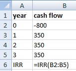
3) PI: profitable index

SO, PI= (350/(1+11%) + 350/(1+11%)2 +
350/(1+11%)3 ) / 800 = 1.069
Or PI = NPV/800 + 1 = 55.30/800 + 1 = 1.069
4) Payback period:

A portion of the third year =
(800-350-350)/350 = 100/350 = 0.2857
So it takes 2 + 0.2857 = 2.2857 years to pay
off the debt of $800.
5) Discounted payback period:
Note: All the cash flows in the above equation
should be the present values.
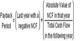
A portion of the third year =
(800-318.18-289.26)/262.96 = 0.72
So it takes 2 + 0.72 = 2.72 years to pay off
the debt of $800.
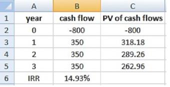
A portion of the third year =
(800-318.18-289.26)/262.96 = 0.72
So it takes 2 + 0.72 = 2.72 years to pay off
the debt of $800.
Or use the calculator at https://www.jufinance.com/capital/
Part II:
Multi-Projects
1. Projects S and L, whose cash flows are shown
below. These projects are mutually exclusive, equally risky, and
not repeatable. The CEO believes the IRR is the best selection
criterion, while the CFO advocates the NPV. If the decision is
made by choosing the project with the higher IRR rather than the one with the
higher NPV, how much, if any, value will be forgone, i.e., what's the chosen
NPV versus the maximum possible NPV? Note that (1) “true
value” is measured by NPV, and (2) under some conditions the choice of
IRR vs. NPV will have no effect on the value gained or lost.
WACC: 7.50%
Year 0 1 2 3 4
CFS -$1,100 $550 $600 $100 $100
CFL -$2,700 $650 $725 $800 $1,400
Answer:
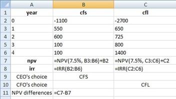
Question 2:
|
Period |
Project A |
Project B |
|
0 |
-500 |
-400 |
|
1 |
325 |
325 |
|
2 |
325 |
200 |
|
IRR |
||
|
NPV |
If the required rate of return is 10%. Which project shall you
choose?
1) How
much is the cross over rate? (answer: 11.8%)
2) How
is your decision if the required rate of return is 13%? (answer: NPV of
B>NPV of A)
· Rule for mutually exclusive projects: (answer:
Choose B)
· What about the two projects are independent? (answer:
Choose both)
Solution:

Part III More on
IRR – (non-conventional cash flow)
Suppose an investment will cost $90,000
initially and will generate the following cash flows:
– Year 1: 132,000
– Year 2: 100,000
– Year 3: -150,000
The required return is 15%. Should we accept
or reject the project?
1) How does the
NPV profile look like? (Answer: Inverted NPV profile)
2) IRR1= 10.11% --
answer
3) IRR2= 42.66% --
answer
Solution:

Class Video of
Chapter 11’s Case Study
Modified
Internal Rate of Return (MIRR)
By ADAM HAYES Updated June
12, 2022 Reviewed by DAVID KINDNESS Fact checked by JIWON MA
Video https://www.investopedia.com/terms/m/mirr.asp
What Is
Modified Internal Rate of Return (MIRR)?
The modified internal
rate of return (MIRR) assumes that positive cash flows are reinvested at the
firm's cost of capital and that the initial outlays are financed at the
firm's financing cost. By contrast,
the traditional internal rate of return (IRR) assumes the cash flows from a
project are reinvested at the IRR itself. The MIRR, therefore, more
accurately reflects the cost and profitability of a project.
Meanwhile, the internal rate of return (IRR) is a discount rate
that makes the net present value (NPV) of all cash flows from a particular
project equal to zero. Both MIRR and IRR calculations rely on the formula for
NPV.
KEY TAKEAWAYS
·
MIRR improves on IRR by
assuming that positive cash flows are reinvested at the firm's cost of
capital.
·
MIRR is used to rank investments
or projects a firm or investor may undertake.
·
MIRR is designed to generate
one solution, eliminating the issue of multiple IRRs.
What MIRR Can Tell You
The MIRR is used
to rank investments or projects of unequal size. The calculation is a solution to two major problems that exist
with the popular IRR calculation. The first main problem with IRR is that
multiple solutions can be found for the same project. The second problem is
that the assumption that positive cash flows are reinvested at the IRR is
considered impractical in practice. With the MIRR, only a single solution
exists for a given project, and the reinvestment rate of positive cash flows
is much more valid in practice. The MIRR allows project managers to change
the assumed rate of reinvested growth from stage to stage in a project. The
most common method is to input the average estimated cost of capital, but
there is flexibility to add any specific anticipated reinvestment rate.
The Difference
Between MIRR and IRR
Even though the internal rate
of return (IRR) metric is popular among business managers, it tends to
overstate the profitability of a project and can lead to capital budgeting
mistakes based on an overly optimistic estimate. The modified internal
rate of return (MIRR) compensates for this flaw and gives managers more
control over the assumed reinvestment rate from future cash flow. An IRR
calculation acts like an inverted compounding growth rate. It has to discount
the growth from the initial investment in addition to reinvested cash flows.
However, the IRR does not paint a realistic picture of how cash flows are
actually pumped back into future projects. Cash flows are often reinvested at
the cost of capital, not at the same rate at which they were generated in the
first place. IRR assumes that the growth rate remains constant from project
to project. It is very easy to overstate potential future value with basic
IRR figures. Another major issue with IRR occurs when a project has different
periods of positive and negative cash flows. In these cases, the IRR produces
more than one number, causing uncertainty and confusion. MIRR solves this
issue as well.
Limitations of Using MIRR
The first
limitation of MIRR is that it requires you to compute an estimate of the cost
of capital in order to make a decision, a calculation that can be subjective
and vary depending on the assumptions made. As with IRR, the MIRR can provide information that leads to
sub-optimal decisions that do not maximize value when several investment options
are being considered at once. MIRR does not actually quantify the various
impacts of different investments in absolute terms; NPV often provides a more effective theoretical basis for selecting
investments that are mutually exclusive. It may also fail to produce
optimal results in the case of capital rationing. MIRR can also be difficult
to understand for people who do not have a financial background. Moreover,
the theoretical basis for MIRR is also disputed among academics.
In Class Exercise (FYI) MIRR Quiz here
1. What does MIRR improve upon compared to IRR?
A) Multiple solutions for the same project
B) Reinvestment rate assumption
C) Discount rate calculation
Answer: B
Explanation: MIRR improves upon IRR by addressing the
unrealistic assumption of reinvesting cash flows at the IRR itself.
2. What does MIRR allow project managers to do?
A) Change reinvestment rate assumptions
B) Assume reinvestment rate at IRR
C) Use NPV calculations exclusively
Answer: A
Explanation: MIRR allows project managers to adjust
the assumed reinvestment rate, providing flexibility in modeling different
scenarios.
3. How does IRR tend to overstate project profitability?
A) By assuming reinvestment at cost of capital
B) By discounting future cash flows
C) By considering multiple reinvestment rates
D) None of the above
Answer: D
Explanation: IRR tends to overstate project
profitability due to unrealistic assumptions about reinvestment rates.
4. When is MIRR particularly useful?
A) When project cash flows are unpredictable
B) When all projects have the same reinvestment rate
C) When comparing projects of unequal size
Answer: C
Explanation: MIRR is particularly useful when
evaluating projects with different sizes and cash flow patterns.
5. What is the key difference between MIRR and IRR?
A) MIRR accounts for project size
B) MIRR assumes reinvestment at cost of capital
C) MIRR eliminates the issue of multiple solutions
Answer: B
Explanation: MIRR assumes reinvestment of positive
cash flows at the cost of capital, while IRR assumes reinvestment at the IRR
itself.
6. Which metric is more likely to lead to capital budgeting
mistakes based on overly optimistic estimates?
A) MIRR
B) NPV
C) IRR
Answer: C
Explanation: IRR tends to overstate project
profitability and can lead to capital budgeting mistakes based on overly
optimistic estimates.
7. What problem does MIRR solve related to IRR when a project
has different periods of positive and negative cash flows?
A) Inconsistent reinvestment rates
B) Multiple IRRs
C) Overstated profitability
Answer: B
Explanation: MIRR generates one solution for a given
project, eliminating the issue of multiple IRRs.
8. Which metric is more effective in selecting mutually
exclusive investments?
A) MIRR
B) NPV
C) IRR
Answer: B
Explanation: NPV often provides a more effective
theoretical basis for selecting mutually exclusive investments.
Second Midterm
Exam (3.21, in class exam)
·
Chapters 9, 10, 11
·
similar to in class
exercises and case studies
What is DCF?
Video – Amazon
– DCF Example (self-made video in
spring 2023)
Evaluation of Amazon
based on DCF – ChatGPT done in Spring
2023
DCF (Discounted Cash Flow) analysis is a commonly used method
for evaluating the intrinsic value of a company. It is based on the idea that
the value of a company is determined by the present value of its expected
future cash flows.
Here are the steps to evaluate Amazon using DCF:
Step 1: Estimate Amazon's
Free Cash Flow (FCF)
FCF is the cash generated by a company after accounting for
all capital expenditures needed to maintain or grow the business. To calculate
Amazon's FCF, we can start with its operating cash flow and subtract its
capital expenditures.
Operating cash flow for the last 12 months (as of September
2021) was $92.5 billion, and capital expenditures were $24.5 billion.
Therefore, Amazon's FCF is:
FCF = Operating cash flow - Capital expenditures
FCF = $92.5 billion - $24.5 billion
FCF = $68 billion
Step 2: Estimate Amazon's
growth rate
Next, we need to estimate the rate at which Amazon's FCF is
likely to grow in the future. One way to do this is to look at the historical
growth rates and make an educated guess about future growth.
Amazon's FCF has grown at an average rate of 25% over the past
five years. Assuming a conservative growth rate of 15% for the next five
years, and then a terminal growth rate of 3% after that, we can estimate
Amazon's future FCF as follows:
Year 1 FCF = $68 billion x (1 + 15%) = $78.2 billion
Year 2 FCF = $78.2 billion x (1 + 15%) = $89.9 billion
Year 3 FCF = $89.9 billion x (1 + 15%) = $103.4 billion
Year 4 FCF = $103.4 billion x (1 + 15%) = $119 billion
Year 5 FCF = $119 billion x (1 + 15%) = $137 billion
Terminal FCF = $137 billion x (1 + 3%) / (11% - 3%) = $1760.94
billion (11% is the WACC)
Step 3: Determine Amazon's
Discount Rate
The discount rate is the rate of return required by investors
to compensate for the risk of investing in a company. A higher discount rate
indicates a higher level of risk. To determine Amazon's discount rate, we can
use the CAPM (Capital Asset Pricing Model), which takes into account the
risk-free rate, market risk premium, and Amazon's beta.
Assuming a risk-free rate of 2%, a market risk premium of 6%,
and Amazon's beta of 1.5, we can calculate Amazon's discount rate as follows:
Discount rate = Risk-free rate + Beta x Market risk premium
Discount rate = 2% + 1.5 x 6%
Discount rate = 11%
Step 4: Calculate Amazon's
Intrinsic Value
Finally, we can calculate Amazon's intrinsic value using the
discounted cash flow formula, which is the sum of the present value of all
future cash flows.
Intrinsic value = (Year 1 FCF / (1 + Discount rate)^1) + (Year
2 FCF / (1 + Discount rate)^2) + ... + (Terminal FCF / (1 + Discount rate)^5)
Intrinsic value = ($78.2 billion / (1 + 11%)^1) + ($89.9
billion / (1 + 11%)^2) + ($103.4 billion / (1 + 11%)^3) + ($119 billion / (1
+ 11%)^4) + ($137 billion / (1 +11%)^5) + ($1.76 trillion / (1 + 11%)^5)
Intrinsic value = $1,423 billion
We made the assumption that AMAZON's cost of equity is roughly
equivalent to its WACC for the purpose of simplifying the calculation.
However, according to gurufocus.com, as of the end of March 2023, AMAZON's
WACC is 9.65%.
Step 5: Compare Intrinsic
Value with Market Value
The last step is to compare the intrinsic value we calculated
with the current market value of Amazon. As of March 2023, Amazon's market
capitalization is around $2.4 trillion.
Comparing the intrinsic value of $1,423 billion with the
market capitalization of $2.4 trillion, we can see that the market value is
higher than the intrinsic value, which suggests that the stock may be
overvalued. However, it's important to keep in mind that the DCF analysis is
based on various assumptions and estimates, and the actual value of a company
may differ from the calculated intrinsic value.
Therefore, it's important to use multiple valuation methods
and take into account other factors such as industry trends, competitive
landscape, and management quality to make an informed investment decision.
To calculate the estimated per-share stock price based on the
DCF analysis, we can divide the intrinsic value by the total number of shares
outstanding. As of December 2021, Amazon had around 500 million shares
outstanding.
Estimated Per-Share Stock Price = Intrinsic Value / Shares
Outstanding
Estimated Per-Share Stock Price = $1,423 billion / 500 million
Estimated Per-Share Stock Price = $2,847
Therefore, based on this DCF analysis, the estimated per-share
stock price for Amazon is $2,847. However, it's important to note that this
is just an estimate based on certain assumptions and estimates, and the
actual stock price may differ based on various factors such as market
sentiment, company performance, and global economic conditions.
Step one of DCF: FCF -
Chapter 3 Financial Statement
Balance Sheet Template https://www.jufinance.com/10k/bs
Income Statement Template https://www.jufinance.com/10k/is
Cash flow template https://www.jufinance.com/10k/cf
Note:
All companies, foreign and domestic, are required to file registration
statements, periodic reports, and other forms electronically through
EDGAR.
************
What
is Free Cash Flow **************
What is free cash flow (video)
What is free cash flow (FCF)? Why is it
important?
•
FCF is the amount of cash available from
operations for distribution to all investors (including stockholders
and debt holders) after making the necessary
investments to support operations.
•
A company’s value depends on the amount of
FCF it can generate.
What are the five uses
of FCF?
o
Pay interest on debt.
o
Pay back principal on debt.
o
Pay dividends.
o
Buy back stock.
o
Buy non-operating assets
(e.g., marketable securities, investments in other companies, etc.)
In class exercise
Firm AAA has EBIT (operating income) of $3
million, depreciation of $1 million. Firm AAA’s expenditures
on fixed assets = $1 million. Its net operating working capital = $0.6
million. Calculate for free cash flow. Imagine that the tax rate
=40%.
FCF = EBIT(1
– T) + Deprec. – (Capex + NOWC)
answer:
EBIT $3
Tax
rate 40%
Depreciation $1
Capex + NOWC $1.60
So, FCF = 3*(1-40%) + 1 –(1+0.6) =
1.2
Case study of
chapter 3 on Cash Flow Statement and FCF only (due with final)
A review of Cash Flow Statement (FIN301): https://www.jufinance.com/10k/cf/
|
Cash Flow Statement |
Notes |
|
|
Cash at the
beginning of the year |
Cash, last year's balance sheet; "=Cash in 2022" |
|
|
Cash From operation |
||
|
net income |
Income statement of 2023 |
|
|
plus depreciation |
Income statement of 2023 |
|
|
-/+ AR |
Changes of AR between this year and last year - balance sheet.
CHANGE SIGN! use 2023 - 2022 |
|
|
-/+ Inventory |
Changes of Inventory between this year and last year ///
balance sheet. CHANGE SIGN! use 2023 - 2022 |
|
|
+/- AP |
Changes of AP between this year and last year /// balance
sheet. use 2023 - 2022 |
|
|
net change in cash from operation |
-- |
|
|
Cash From investment |
||
|
-/+ (NFA+depreciation) |
Changes of NFA between this year & last year, add back
depreciation//balance sheet. CHANGE SIGN! |
|
|
net change in cash from investment |
-- |
|
|
Cash From Financing |
||
|
+/- long term debt |
Changes of LD between this year and last year /// balance
sheet. use 2023 - 2022 |
|
|
Common stock |
Changes of CS between this year and last year /// balance
sheet. use 2023 - 2022 |
|
|
- dividend |
Income statement of 2023; Do not add negative sign to subtract
dividend |
|
|
net change in cash from financing |
-- |
|
|
Total net change of cash |
-- |
|
|
Cash at the end of the year |
-- |
Should match Cash on
current year's balance sheet; if not, go back and check;
"=2023's cash" |
Step 2 of DCF - Chapter 12: Cash
Flow Estimation and Monte Carlo Method in Excel
Chapter
12 case study (due with final. Monte
Carol is required.)
Case Video
in Class on 3/28/2024
Monte
Carlo Demonstration Based on Case in Class (FYI, Video)
Critical thinking
challenge (due with final):
· Recalculate 100 times of the NPV based on the Monte Carlo simulation
method by randomly changing the tax rate and the WACC (or any two factors)
· Report
statistical results: Mean, Standard Deviation, Min, Max of the NPV.
· Report the
Histogram of the NPV, or the probability distribution of the NPV, such as the
following:
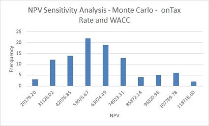
Instructions on Monte Carlo Simulation Process (using Tax Rate and WACC
as example):
· Pick two variables, such as tax rate and WACC.
· Parameter Definition:
You defined the parameters for the two variables, such as tax rate and WACC, including their means and standard deviations.
· Random Sample Generation: Using the norminv function, you generated 100 sets of random samples for tax rate and WACC, ensuring they follow normal distributions based on the provided mean and standard deviation.
· NPV Calculation: For each set of randomly generated tax rate and WACC, you calculated the Net Present Value (NPV) using the appropriate formula.
· Statistical Analysis: You reported statistical results including the mean, standard deviation, minimum, and maximum NPV values obtained from the Monte Carlo simulation.
· Histogram Visualization: You visualized the probability distribution of NPV values by creating a histogram.
· Summary of Results:
Mean NPV: The
average NPV across the 100 iterations.
Standard
Deviation of NPV: The measure of dispersion of NPV values around the mean.
Minimum NPV:
The lowest NPV value obtained.
Maximum NPV:
The highest NPV value obtained.
Histogram: The
histogram provides a visual representation of the distribution of NPV values,
showing the frequency of NPV occurrences within different ranges.
· Conclusion:
Your Monte
Carlo simulation approach effectively captured the variability and
uncertainty in NPV outcomes resulting from fluctuations in tax rates and
WACC. The statistical analysis and histogram visualization offer insights
into the range of potential NPV values and their likelihood of occurrence,
aiding in decision-making processes related to financial planning and
investment evaluation.
About norminv
function in excel: =norminv(RAND(), mean, standard_deviation)
· RAND() generates a random number between 0 and 1.
· For example, to generate a random tax rate with a mean of 25% and a standard deviation of 2.5%, you can use:
=norminv(RAND(),
25%, 2.5%)
Monte Carlo
Simulation Demonstration (FYI,
2023 video)
Introduction to
Monte Carlo Simulation in Excel 2016 (youtube)
|
Structure |
|
|||||||||||
|
|
|
|
|
|
|
|||||||
|
0 |
1 |
2 |
3 |
4 |
||||||||
|
Investment Outlay |
||||||||||||
|
Equipment
cost |
$(----------) |
|||||||||||
|
Installation |
(--------) |
|||||||||||
|
Increase
in inventory |
(-------) |
|||||||||||
|
Increase
in A/P |
------- |
|||||||||||
|
Initial
net investment |
$(-------) |
|||||||||||
|
Operating Cash Flows |
||||||||||||
|
Units
sales |
------- |
------- |
------- |
------- |
||||||||
|
Price
per unit |
*
$ --- |
$ --- |
$ --- |
$ --- |
||||||||
|
Total
revenues |
------- |
------- |
------- |
------- |
||||||||
|
Operating
costs (w/o deprn) |
------- |
------- |
------- |
------- |
||||||||
|
Depreciation |
------- |
------- |
------- |
------- |
||||||||
|
Total
costs |
------- |
------- |
------- |
------- |
||||||||
|
Operating
income |
------- |
------- |
------- |
------- |
||||||||
|
Taxes
on operating income |
------- |
------- |
------- |
------- |
||||||||
|
A-T
operating income |
------- |
------- |
------- |
------- |
||||||||
|
Depreciation |
------- |
------- |
------- |
------- |
||||||||
|
Operating
cash flow |
------- |
------- |
------- |
------- |
||||||||
Terminal Year Cash
Flows
Recovery of net
working capital
-------
|
Salvage
value |
------- |
||||||||||
|
Tax
on salvage value |
(-------) |
||||||||||
|
Total
termination cash flow |
------- |
||||||||||
|
Project Cash Flows |
|
|
|
|
|
||||||
|
Net
cash flows |
$(-------) |
$ ------- |
$ ------- |
$ ------- |
||||||||
In class exercise (self-study)
1. What is the project's Year 1 cash
flow?
Sales revenues $22,250
Depreciation $8,000
Other operating costs $12,000
Tax rate 35.0%
Answer:
Sales revenues $22,250
− Operating costs (excl. deprec.) 12,000
− Depreciation 8,000
Operating income (EBIT) $ 2,250
−
Taxes Rate = 35% 788
After-tax EBIT $ 1,463
+
Depreciation 8,000
Cash
flow, Year 1 $ 9,463
2. The required equipment has a 3-year
tax life, and it will be depreciated by the straight-line method over 3
years. What is the project's Year 1
cash flow?
Equipment cost (depreciable basis) $65,000
Straight-line depreciation rate 33.333%
Sales revenues, each year $60,000
Operating costs (excl. deprec.) $25,000
Tax rate 35.0%
Answer:
Equipment life, years 3
Equipment cost $65,000
Depreciation: rate = 33.333% $21,667
Sales revenues $60,000
− Basis x rate =
depreciation 21,667
− Operating costs (excl. deprec.)
25,000
Operating income (EBIT) $13,333
− Taxes Rate
= 35.0% 4,667
After-tax EBIT $ 8,667
+
Depreciation 21,667
Cash
flow, Year 1 $30,333
3. The equipment that would be used
has a 3-year tax life, and the allowed depreciation rates for such property
are 33%, 45%, 15%, and 7% for Years 1 through 4. Revenues and other operating costs are
expected to be constant over the project's 10-year expected life. What is the Year 1 cash flow?
Equipment cost (depreciable basis) $65,000
Sales revenues, each year $60,000
Operating costs (excl. deprec.) $25,000
Tax rate 35.0%
Answer:
Equipment cost $65,000
Depreciation rate 33.0%
Sales revenues $60,000
− Operating costs (excl. deprec.) 25,000
− Depreciation 21,450
Operating income (EBIT) $13,550
−
Taxes Rate = 35% 4,743
After-tax EBIT $ 8,808
+
Depreciation 21,450
Cash
flow, Year 1 $30,258
4. The equipment that would be used
has a 3-year tax life, would be depreciated by the straight-line method over
its 3-year life, and would have a zero salvage value. No new working capital would be
required. Revenues and other operating
costs are expected to be constant over the project's 3-year life. What is the project's NPV?
Risk-adjusted WACC 10.0%
Net investment cost (depreciable
basis) $65,000
Straight-line deprec. rate 33.3333%
Sales revenues, each year $65,500
Operating costs (excl. deprec.),
each year $25,000
Tax rate 35.0%
Answer:
WACC 10.0% Years 0 1 2 3
Investment cost -$65,000
Sales revenues $65,500 $65,500 $65,500
− Operating costs (excl. deprec.) 25,000 25,000 25,000
− Depreciation rate = 33.333% 21,667 21,667 21,667
Operating income (EBIT) $18,833 $18,833 $18,833
−
Taxes Rate = 35% 6,592 6,592 6,592
After-tax EBIT $12,242 $12,242 $12,242
+
Depreciation 21,667
21,667 21,667
Cash flow -$65,000 $33,908 $33,908 $33,908
NPV $19,325
5. The equipment originally cost
$22,500, of which 75% has been depreciated.
The firm can sell the used equipment today for $6,000, and its tax
rate is 40%. What is the equipment’s
after-tax salvage value for use in a capital budgeting analysis? Note that if the equipment's final market
value is less than its book value, the firm will receive a tax credit as a
result of the sale.
Answer:
% depreciated on equip. 75%
Tax rate 40%
Equipment cost $22,500
− Accumulated deprec. 16,875
Current book value of equipment $ 5,625
Market value of equipment 6,000
Gain (or loss): Market value − Book value $
375
Taxes paid on gain (−) or
credited (+) on loss -150
AT
salvage value = market value +/− taxes $
5,850
The Monte Carlo Simulation: Understanding the
Basics (FYI)
By KUSHAL AGARWAL Updated June 19, 2023
What
Is a Monte Carlo Simulation?
Analysts can assess possible portfolio
returns in many ways. The historical approach, which is the most popular,
considers all the possibilities that have already happened. However,
investors shouldn't stop at this. The
Monte Carlo method is a stochastic (random sampling of inputs) method to
solve a statistical problem, and a simulation is a virtual representation
of a problem. The Monte Carlo
simulation combines the two to give us a powerful tool that allows us to
obtain a distribution (array) of results for any statistical problem with
numerous inputs sampled over and over again.
KEY TAKEAWAYS
· The Monte Carlo method uses a random sampling of information to solve a statistical problem; while a simulation is a way to virtually demonstrate a strategy.
· Combined, the Monte Carlo simulation enables a user to come up with a bevy of results for a statistical problem with numerous data points sampled repeatedly.
· The Monte Carlo simulation can be used in corporate finance, options pricing, and especially portfolio management and personal finance planning.
· On the downside, the simulation is limited in that it can't account for bear markets, recessions, or any other kind of financial crisis that might impact potential results.
Monte
Carlo Simulation Demystified
Monte Carlo simulations can be best understood
by thinking about a person throwing dice. A novice gambler who plays craps
for the first time will have no clue what the odds are to roll a six in any
combination (for example, four and two, three and three, one and five). What
are the odds of rolling two threes, also known as a "hard six?" Throwing the dice many times, ideally
several million times, would provide a representative distribution of
results, which will tell us how likely a roll of six will be a hard six. Ideally,
we should run these tests efficiently and quickly, which is exactly what a
Monte Carlo simulation offers.
The problem with looking to history alone is
that it represents, in effect, just one roll, or probable outcome, which may
or may not be applicable in the future. A
Monte Carlo simulation considers a wide range of possibilities and helps us
reduce uncertainty. A Monte Carlo simulation is very flexible; it allows
us to vary risk assumptions under all parameters and thus model a range of
possible outcomes. One can compare multiple future outcomes and customize the
model to various assets and portfolios under review.
A
Monte Carlo simulation can accommodate a variety of risk assumptions in many
scenarios and is therefore applicable to all kinds of investments and
portfolios.
Applying
the Monte Carlo Simulation
The Monte Carlo simulation has
numerous applications in finance and other fields. Monte Carlo is used in corporate finance to model components of
project cash flow, which are impacted by uncertainty. The result is a range
of net present values (NPVs) along with observations on the average NPV of
the investment under analysis and its volatility. The investor can, thus, estimate the probability that NPV will be
greater than zero. Monte Carlo is
used for option pricing where numerous random paths for the price of an
underlying asset are generated, each having an associated payoff. These
payoffs are then discounted back to the present and averaged to get the
option price. It is similarly used for pricing fixed income securities and
interest rate derivatives. But the Monte Carlo simulation is used most
extensively in portfolio management and personal financial planning.
Uses
in Portfolio Management
A
Monte Carlo simulation allows an analyst to determine the size of the portfolio
a client would need at retirement to support their desired retirement
lifestyle and other desired gifts and bequests. She factors
into a distribution of reinvestment rates, inflation rates, asset class
returns, tax rates, and even possible lifespans. The result is a distribution
of portfolio sizes with the probabilities of supporting the client's desired
spending needs.
The analyst next uses the Monte Carlo
simulation to determine the expected value and distribution of a portfolio at
the owner's retirement date. The simulation allows the analyst to take a
multi-period view and factor in path dependency; the portfolio value and
asset allocation at every period depend on the returns and volatility in the
preceding period. The analyst uses various asset allocations with varying
degrees of risk, different correlations between assets, and distribution of a
large number of factors – including the savings in each period and the
retirement date – to arrive at a distribution of portfolios along with the
probability of arriving at the desired portfolio value at retirement. The
client's different spending rates and lifespan can be factored in to
determine the probability that the client will run out of funds (the
probability of ruin or longevity risk) before their death.
A client's risk and return profile is
the most important factor influencing portfolio management decisions. The
client's required returns are a function of her retirement and spending
goals; her risk profile is determined by her ability and willingness to take
risks. More often than not, the desired return and the risk profile of a
client are not in sync with each other. For example, the level of risk
acceptable to a client may make it impossible or very difficult to attain the
desired return. Moreover, a minimum amount may be needed before retirement to
achieve the client's goals, but the client's lifestyle would not allow for
the savings or the client may be reluctant to change it.
Monte
Carlo Simulation Example
Let's consider an example of a young
working couple who works very hard and has a lavish lifestyle including
expensive holidays every year. They have a retirement objective of spending
$170,000 per year (approx. $14,000/month) and leaving a $1 million estate to
their children. An analyst runs a simulation and finds that their
savings-per-period is insufficient to build the desired portfolio value at
retirement; however, it is achievable if the allocation to small-cap stocks
is doubled (up to 50 to 70% from 25 to 35%), which will increase their risk
considerably. None of the above alternatives (higher savings or increased
risk) are acceptable to the client. Thus, the analyst factors in other
adjustments before running the simulation again. the analyst delays their
retirement by two years and decreases their monthly spend post-retirement to
$12,500. The resulting distribution shows that the desired portfolio value is
achievable by increasing allocation to small-cap stock by only 8 percent.
With the available insight, the analyst advises the clients to delay
retirement and decrease their spending marginally, to which the couple
agrees.
The
Bottom line
A Monte Carlo simulation allows
analysts and advisors to convert investment chances into choices. The
advantage of Monte Carlo is its ability to factor in a range of values for
various inputs; this is also its greatest disadvantage in the sense that
assumptions need to be fair because the output is only as good as the inputs.
Another great disadvantage is that the
Monte Carlo simulation tends to underestimate the probability of extreme bear
events like a financial crisis. In fact, experts argue that a simulation like
the Monte Carlo is unable to factor in the behavioral aspects of finance and
the irrationality exhibited by market participants. It is, however, a useful
tool for advisors.
In
Class Exercise (FYI)
1.
What does the Monte Carlo simulation involve?
a)
Generating random paths for the price of an underlying asset
b)
Analyzing historical data only
c)
Calculating deterministic outcomes
Answer: a
Explanation: The Monte Carlo simulation involves generating random paths for the
price of an underlying asset to analyze a range of possible outcomes.
2.
In finance, Monte Carlo simulation is primarily used for:
a)
Analyzing historical trends
b)
Predicting deterministic outcomes
c)
Portfolio management and personal financial planning
Answer: c
Explanation: Monte Carlo simulation is extensively used in portfolio management
and personal financial planning to assess various outcomes and risks.
3.
What does the Monte Carlo simulation allow an analyst to determine in
portfolio management?
a) The
exact portfolio size needed at retirement
b) The
expected value and distribution of a portfolio at a specific date
c) The
precise returns of individual assets
Answer: b
Explanation:
In portfolio management, the Monte Carlo simulation allows an analyst to
determine the expected value and distribution of a portfolio at a specific
date.
4.
What is the key factor influencing portfolio management decisions in Monte
Carlo simulations?
a)
Inflation rates
b) Risk
and return profile of the client
c) Tax
rates
Answer: b
Explanation: The risk and return profile of the client is the key factor
influencing portfolio management decisions in Monte Carlo simulations.
5.
What is the greatest disadvantage of Monte Carlo simulation?
a)
Inability to factor in market irrationality
b)
Overestimation of extreme bear events
c)
Underestimation of extreme bear events
Answer: c
Explanation: The greatest disadvantage of Monte Carlo simulation is its tendency
to underestimate the probability of extreme bear events like a financial
crisis.
6.
How does a Monte Carlo simulation help convert investment chances into
choices?
a) By
eliminating all risks
b) By
considering a range of values for various inputs
c) By
providing deterministic outcomes
Answer: b
Explanation: A Monte Carlo simulation helps convert investment chances into
choices by considering a range of values for various inputs, allowing for
better decision-making.
7.
What is the main advantage of Monte Carlo simulation?
a) It
provides deterministic outcomes
b) It
factors in market irrationality
c) It
considers a range of values for various inputs
Answer: c
Explanation: The main advantage of Monte Carlo simulation is its ability to
consider a range of values for various inputs, allowing for comprehensive
analysis.
8.
What is the primary application of Monte Carlo simulation in corporate
finance?
a)
Analyzing historical trends
b)
Pricing fixed income securities
c) Portfolio
management and personal financial planning
d)
Modeling components of project cash flow in corporate finance
Answer: d
Explanation: In addition to portfolio management and personal financial planning,
Monte Carlo simulation is widely used in corporate finance for modeling
components of project cash flow, especially those impacted by uncertainty.
Chapter 19 Derivatives
Chapter 19 Case Study
Part I - due with final
Chapter 19 Case
Study part II – due with final
Case video in class
Part I (4.9.2024) – Black-Schools-Merton Option Pricing Model
Case video in class
part II (4.11.2024) – Binomial Option Pricing Model
1st, understand what is call and put
option
2nd,
understand the pay off of call and put option
3rd,
can draw payoff profile of call and put option
Call
and Put Option Calculator
www.jufinance.com/option
Call and Put Option Diagram Illustration Excel
(Thanks to
Dr. Greence at UAH)
4th, can calculate call option
pricing using binomial model
Binomial Calculator by ChatGPT
Instruction on Binomial
model - in class exercise - case study
·
In the first step, you are calculating the
range of values at expiration by considering the two possible ending stock prices
of $30 and $50. You then calculate the ending option and portfolio values for
each of these stock prices.
·
Next, in step 2, you are equalizing the
range of payoffs for the stock and the option by buying 0.75 shares and selling 1 option.
This allows you to create a riskless hedged investment in step 3, where you
calculate the ending values of the portfolio for the two possible ending
stock prices.
·
Finally, in step 4, you are pricing the
call option by calculating the present value of the portfolio using the
risk-free rate of 8%. The calculated present value of the portfolio is
$20.83, which can be used to calculate the call option value.
5th, can calculate call
option price using black-scholes model
Black-Scholes-Merton Option
Calculator
https://www.mystockoptions.com/black-scholes.cfm
or
Black-Scholes-Merton Option
Calculator by ChatGPT (at
jufinance.com)
www.jufinance.com/https://www.jufinance.com/option_chatgpt/
Black-Scholes-Merton Model
Illustration Excel
Binomial Option Pricing Model Explained ----
using In Class Case Study as an example (FYI only)
The
binomial option pricing model is a mathematical formula that allows us to calculate
the fair value of an option by modeling the possible future prices of the
underlying asset, and calculating the probability of each price occurring.
The model works by
creating a binomial tree that represents the possible future prices of the asset,
and then working backward through the tree to calculate the expected value of
the option at each node.
Here
are the steps to use the binomial option pricing model:
Step 1: Determine the
Inputs
The
first step is to gather the inputs needed for the model. These include:
·
The current price of the underlying asset
·
The range of possible future prices of the
asset
·
The exercise price of the option
·
The risk-free rate of interest
·
The time until expiration of the option
Let’s
try to work on the same question as we did in class. A stock that is currently trading at $40, and two possible future
prices at the end of one year are: $30 and $50. The exercise price of the
option is $35, the risk-free rate is 8%, and the time until expiration is one
year --- our case study example
Step 2: Calculate the Up
and Down Factors
The
next step is to calculate the up and down factors, which represent the
expected percentage increase and decrease in the stock price over one period.
These factors are calculated as:
·
Up factor (u) = Future price if stock goes
up / Current stock price
·
Down factor (d) = Future price if stock
goes down / Current stock price
In
our example, the up factor is $50 /
$40 = 1.25, and the down factor is $30 / $40 = 0.75.
Step 3: Create the Binomial
Tree
This
step involves creating the binomial tree as below.
Binomial Tree
$40
/
\
$50
$30
Step 4: Calculate the
Risk-Neutral Probability
The
next step is to calculate the probability of each future price occurring,
using the risk-neutral probability. The
risk-neutral probability is the probability of the stock going up or down,
assuming that the market is risk-neutral and the expected return of the stock
is equal to the risk-free rate.
The
risk-neutral probability is calculated as:
Risk-neutral probability
(p) = (1+r*t - d)/(u-d)
where
r is the risk-free rate and t is the time until expiration; u is
the up factor and d is the down factor.
In
our example, the risk-neutral probability is approximately:
Pu = (1+0.08*1 -
0.75)/(1.25-0.75)= 0.66
Or
use the more accurate model:
Risk-neutral
probability Pu = (e^((r * t)/n) - d) / (u - d)
where
r is the risk-free rate and t is the time until expiration, and n is the
height of the binomial tree. In our example, n=1.
In
our example, the risk-neutral probability is:
Pu
= (e^(0.08 * 1) - 0.75) / (1.25 - 0.75) = 0.6666
Step 5: Calculate the Option
Value at Each Node of the Tree
To
get the value of the option at each node of the tree, we should work backward
from the end of the tree to the current price of the stock.
Simply
speaking, at the end of the tree, the option value = difference between the
stock price and the exercise price, or zero if the stock price is below the
exercise price.
For
example, we need to calculate the value of the option if the stock price goes
up to $50, and if it goes down to $30. The results are as follows.
Vu
= Max($50 - $35, 0) = $15
Vd
= $0
Working
backward up the tree, we can calculate the option value at each node as the discounted
expected value of the option at the next period:
Option
value = v = (Pu * Vu + Pd * Vd) / (1 + r)^t;
Option
Value at $40 = (0.66 x $15 + (1 - 0.66) x $0) / (1 + 0.08)^1 = $9.17
Therefore,
the value of the option is approximately $9.17 if the stock price is $40.
Black-Scholes-Merton Option Pricing Model
Explained ----
using In Class Case Study as an example (FYI only)
C = SN(d1) –
X*exp(-r*t)*N(d2)
where:
·
S
= the current stock price
·
X
= the option strike price
·
r
= the risk-free interest rate
·
t
= time until expiration, expressed as a fraction of a year
|
V = |
P[
N (d1) ] − Xe-rRF t [ N (d2) ] |
||||
|
d1 = |
{
ln (P/X) + [rRF + s2 /2) ] t } / s (t1/2) |
||||
|
d2
= |
d1
− s (t 1 / 2) |
||||
d1 = [ln(S/X) + (r + σ^2/2)t] / [σsqrt(t)]
d2 = d1 - σ*sqrt(t)
σ
= the annualized standard deviation of stock returns
Using
the values used in the case study in class:
·
S
= X = 21
·
r
= 0.05
·
σ
= 0.3
·
t
= 0.36
First,
we calculate d1 and d2:
d1 =
ln(21/21)+(0.05+0.3^2/2)*0.36)/(0.3*sqrt(0.36)) =0.19
d2 =
0.19 - 0.3*sqrt(0.36) = 0.01
Next,
we calculate the call option price using the Black-Scholes formula:
C = SN(d1) –
X*exp(-r*t)*N(d2)
C = 21*normdist(0.19,
0, 1, true) - 21*exp(-0.05*0.36)*normdist(0.01, 0, 1, true) = 1.687 (rounded
to three decimal places)
Therefore,
the expected result for the call option price using
the Black-Scholes formula with the given inputs is
approximately 1.687.
By the
way, based on Put - Call Parity, the put option price (P) is the following:
P = C - S +
Xe^(-rt)
= 1.687
- 21 + 21*exp(-0.05*0.36) = 1.3124
FYI – normdist
function in Excel
The normdist
function is used in Excel to calculate the probability density function of a
normally distributed random variable. This function takes four arguments: x,
mean, standard_dev, and cumulative.
Here is
a brief explanation of each argument:
·
x:
This is the value for which you want to calculate
the probability density function. It must be a numeric value.
·
mean: This is the mean
of the distribution. It must be a numeric value.
·
standard_dev: This is
the standard deviation of the distribution. It must be a numeric value.
·
cumulative: This is an
optional argument that specifies whether you want to calculate the cumulative
distribution function or the probability density function. If this argument
is omitted or set to TRUE, the function will calculate the cumulative
distribution function. If it is set to FALSE, the function will calculate the
probability density function.
To use the normdist function in Excel, follow these steps:
.
·
In a cell, type
=NORMDIST(x, mean, standard_dev, cumulative) and replace the values of x,
mean, standard_dev, and cumulative with the values you want to use.
·
Press Enter. Excel will
calculate the probability density function or the cumulative distribution
function of the normally distributed random variable, depending on the value of
the cumulative argument.
For example,
1)
if you want to calculate
the probability density function of a normally distributed random variable
with a mean of 10 and a standard deviation of 2 at the value of 12, use the
following: =NORMDIST(12, 10, 2, FALSE) = probability density at that point.
2) =NORMDIST(12, 10, 2, true) calculates the
cumulative distribution function (CDF) of a normally distributed random
variable with a mean of 10 and a standard deviation of 2, evaluated at the
value of 12.
·
The true value of the
fourth argument - calculate the CDF.
Seminar one – Is it
possible for Samsung to acquire Nvidia?
Chapter 21 Mergers and Divestitures
·
This chapter will not be covered in the final
exam
· watch TV series Succession and gain insights of the
dynamics of such corporate fights
Mergers rules of SEC
Mergers are business
combination transactions involving the combination of two or more companies
into a single entity. Most state laws
require that mergers be approved by at least a majority of a company's
shareholders if the merger will have a significant impact on either the
acquiring or target company.
If the company you've
invested in is involved in a merger and is subject to the SEC disclosure
rules, you will receive information about the merger in the form of either
a proxy statement on Schedule 14A or
an information statement on Schedule
14C.
The proxy or information statement will describe the terms of the
merger, including what you will receive if the merger proceeds. If you believe the amount you will
receive is not fair, check the statement for information on appraisal or
dissenter's rights under state law. You must follow the procedures precisely
or your rights may be lost.
You can obtain a copy of a
company's proxy or information statement by using the SEC's EDGAR
database.
Summary
of key M&A documents for finding deal terms of public targets
(www.wsp.com)
|
Acquisition
type |
Document |
Date filed |
Best place to find it |
|
Mergers |
Press release |
Announcement
date |
1. Target (likely also acquirer) will file SEC form
8K (could be in an 8K exhibit) |
|
2. Target (likely also acquirer) website |
|||
|
Mergers |
Definitive agreement |
Announcement
date |
1. Target 8K (often the same 8K that contains press release) |
|
Mergers |
Merger proxy |
Several weeks
after the announcement date |
1. Target PREM14A and DEFM14A |
|
Tender/exchange
offers |
Tender offer (or
exchange offer) |
Upon initiation
of tender offer |
1. Target Schedule TO (attached as exhibit) |
|
|
|||
|
Tender/exchange
offers |
Schedule 14D-9 |
Within 10 days
of filing of Schedule TO |
1. Target Schedule 14D-9 |
|
Mergers and exchange
offers |
Registration
statement/prospectus |
Several weeks
after the announcement date |
1. Acquirer Form S-4 |
******* Whole Foods SEC Filing (FYI)********
Whole foods form 8k filed with SEC on
8/23/2017
“As a result of the Merger, each share of common stock……was
converted into the right to receive $42.00 in cash, without interest (the
“Merger Consideration”).”
Whole Foods DEFA 14A 8k form with SEC 6/14/2017
Whole foods DEFA 14A 8k form with SEC 6/16/2017
Whole foods DEFA 14A 8k form with SEC 6/16/2017
Whole foods is providing materials for the upcoming shareholder
voting.
Whole foods DEFA 14A 8k with SEC 7/21/2017
Has law suit documents
Whole foods DEFA 14A 8k with SEC 7/21/2017
Notifying shareholders for upcoming special shareholder meeting
********* Amazon SEC filing *********
Amazon Form 8k with SEC on 6/15/2017
Financing of the Merger
The Company expects to
finance the Merger with debt financing ……
Amazon Whole Foods Merger Agreement on
6/15/2017
For the term project, if you work on this M&A case, you
should be able to find most of the information in this agreement.
Amazon 8k form Completion of acquisition or
disposition of assets 8/28/2018
********** Miscellaneous **********
7 potential bidders, a call to Amazon, and an
ultimatum: How the Whole Foods deal went down (from business
insider.com)
Final Offer from Amazon: $42/share; a total of
$13.4 billions

Why does
Amazon's Bezos want Whole Foods? (video)
Mergers and
Acquisitions Explained: A Crash Course on M&A (youtube, FYI)
Is it
possible for Samsung to acquire Nvidia?
Samsung
vs. NVIDIA Video produced by invideo.ai and Dr. Foley
IN Class Exercise
1. During the due diligence phase,
Samsung's team primarily focuses on:
a) Assessing financial health
b) Finalizing integration plans
c) Conducting shareholder meetings
Answer:
a
Explanation: Due diligence involves analyzing NVIDIA's
financial health, technology portfolio, market position, and potential
synergies with Samsung's existing businesses.
2. Which of the following is a potential
defense mechanism that NVIDIA's board might employ to deter Samsung's
acquisition attempt?
a) Poison Pill
b) Shareholder approval
c) Regulatory approval
Answer:
a
Explanation: Poison Pill is a defense mechanism used
by companies to dilute the acquirer's stake if it surpasses a certain
threshold, making the acquisition more costly and less attractive.
3. What could be a consequence of NVIDIA
implementing a "poison pill" defense mechanism?
a) Faster acquisition process
b) Shareholder dilution
c) Increased shareholder approval
Answer:
b
Explanation: Implementing a poison pill defense
mechanism could result in diluting the acquirer's stake by issuing additional
shares to existing shareholders.
4. What is one of the strategies NVIDIA's
board could use to counter Samsung's acquisition attempt?
a) Conducting extensive due diligence
b) Offering incentives to key employees
c) Engaging in proxy contests
Answer:
c
Explanation: Proxy contests involve seeking support
from shareholders to vote against the proposed acquisition, highlighting
potential risks or drawbacks associated with Samsung's offer.
5. What regulatory approval might Samsung
need to secure for the acquisition?
a) Shareholder approval
b) Due diligence approval
c) Antitrust approval
Answer:
c
Explanation: Given the size and scope of the two
companies, regulatory approval from various antitrust authorities would be
necessary to ensure the acquisition does not substantially lessen competition
in relevant markets.
6. What action could NVIDIA take if it believes
Samsung's acquisition attempt is unlawful?
a) Shareholder dilution
b) Engaging in litigation
c) Conducting shareholder meetings
Answer:
b
Explanation: NVIDIA could resort to legal action if it
believes Samsung's acquisition attempt is unlawful or not in the best
interests of shareholders.
7. Which of the following is NOT a
potential defense mechanism that NVIDIA's board might employ?
a) Litigation
b) Corporate restructuring
c) Shareholder approval
Answer:
c
Explanation: Shareholder approval is a step in the
acquisition process and not a defense mechanism used by the target company.
8. What role does shareholder approval
play in the acquisition process?
a) It influences the success of the
acquisition
b) It determines the integration timeline
c) It impacts regulatory approval
Answer:
a
Explanation: Shareholder approval is crucial as it
ensures that the acquisition is supported by the company's shareholders,
increasing the likelihood of success.
9. Which defense mechanism involves seeking
out alternative buyers?
a) Poison Pill
b) White Knight
c) Litigation
Answer:
b
Explanation: A white knight is an alternative buyer
sought by the target company to potentially offer a better deal for
shareholders or align more closely with the company's strategic objectives.
10. What could be a consequence of NVIDIA
engaging in litigation against Samsung's acquisition attempt?
a) Delay in regulatory approval
b) Faster integration process
c) Higher shareholder approval
Answer:
a
Explanation: Litigation could lead to delays in the
acquisition process as legal proceedings unfold, potentially delaying
regulatory approval.
11. What could be a consequence of NVIDIA
spinning off certain divisions or assets?
a) Increased shareholder value
b) Delay in shareholder approval
c) Making itself less attractive for
acquisition
Answer:
c
Explanation: Spinning off certain divisions or assets
could make NVIDIA less attractive for acquisition by reducing its overall
value or strategic relevance to the acquirer.
12. What could prolong the process of
replacing NVIDIA's entire board with directors more amenable to the
acquisition?
a) Due diligence
b) Proxy Contest
c) Shareholder approval
Answer:
b
Explanation: Proxy contests involve seeking support
from shareholders to vote against the proposed acquisition, potentially
prolonging the process of replacing the board.
13. What is the primary focus of NVIDIA's
board during a proxy contest?
a) Finalizing integration plans
b) Engaging in litigation
c) Swaying shareholder opinion against the
acquisition
Answer:
c
Explanation: The primary focus of a proxy contest is
to sway shareholder opinion against the acquisition by highlighting potential
risks or drawbacks associated with the offer.
14. What action could Samsung take to
ensure the support and retention of key NVIDIA employees post-acquisition?
a) Offering incentives
b) Engaging in litigation
c) Conducting shareholder meetings
Answer:
a
Explanation: Samsung could offer incentives to key
NVIDIA employees to ensure their support and retention post-acquisition,
aligning their interests with the success of the combined entity.
15. Which defense mechanism involves
making the acquisition more costly and less attractive for the acquirer?
a) White Knight
b) Poison Pill
c) Proxy Contest
Answer:
b
Explanation: Poison Pill defense mechanism aims to
make the acquisition more costly and less attractive for the acquirer by
diluting their stake if
certain thresholds are exceeded.
Self-Test on Merger Knowledge (FYI)
For your knowledge (FYI):
· In
reality, dividends are
more predictable than earnings .
· You own
around 100 shares of the stock of AAA, which is currently being sold for around
$120 per share. A 2-for-1 stock split is about to be declared by the company.
After the split has taken place, which of the following describes your
probable position? You
own 200 shares of AAA’s stock. Meanwhile, the AAA stock price will be near $60
per share.
· Alice
Gordan and Alex Roy believe that when the dividend payout ratio is lowered,
the required return on equity tends to increase. On which of the following
assumptions is their argument based? dividends are viewed as less risky than future capital
gains.
· A
strict residual dividend policy is followed by your firm. Everything remains
constant, which of the factors mentioned below are most probably going to
result in an increase in the dividend per share of a firm? when a company’s profit (net
income) rises
·
Horizontal merger would be an example of The Home Depot and
Lowe’s getting merged.
·
When the merger of two companies in a similar industry takes
place in order to develop products that are needed at various stages of the
production cycle, it is referred to as: integration vertically
.
·
A rights offering that provides the existing target
shareholders with the rights to purchase shares in the acquirer of the target
at an extremely discounted price after particular conditions are met is
referred to as a: poison
pill
(Twitter POISON Pill
Explained by a Lawyer (youtube), FYI)
·
A scenario where each and every director gets a three-year
term to provide their services and the terms are arranged in a staggered
manner so that just one-third of the directors are eligible for the election
every year is referred to as a: classified board
·
In a situation where it becomes inevitable that a hostile
takeover may take place, and a target company may at times search for another
friendlier company in order to acquire it, is referred to as a: white knight
Can Twitter
find a white knight to fend off Elon Musk? (youtube, FYI)
·
When a firm is being taken over and the senior managers of
that firm are let go, a very lucrative severance package is offered to those senior
managers. It is referred to as a: golden parachute
Seminar Two – Which
option should NVIDIA choose: paying dividends or engaging in share
repurchases?
Chapter 15 Distributions to Shareholders
· This
chapter will not be covered in the final exam
Should NVIDIA Pay
Dividends? | Exploring Financial Strategies with Dr. Foley - Made by InVideo.ai
|
Theory |
Explanation |
Alignment with NVIDIA |
|
Residual Theory of Dividends |
Companies should pay dividends only when they have excess
funds after financing all positive NPV projects. |
NVIDIA might not align with this theory as it is a high-growth
technology company that may prioritize reinvesting profits into research
and development, acquisitions, or other growth opportunities over paying
dividends. |
|
Bird-in-Hand Theory |
Investors prefer dividends because they provide a certain
return, while capital gains are uncertain. |
NVIDIA might not align with this theory as it might
prioritize reinvestment to capitalize on growth opportunities, especially
considering its position in the dynamic technology sector. |
|
Clientele Effect |
Companies tend to attract investors with similar preferences
to their dividend policies. |
NVIDIA may align with this theory if it has a significant
portion of investors who prefer capital appreciation over dividends and therefore
chooses not to pay dividends to maintain this investor base. |
|
Signaling Theory |
Paying dividends can signal to investors that a company is
financially healthy and confident about its future prospects. |
NVIDIA might not align with this theory as it might prefer
to reinvest profits rather than signal financial health through dividend
payments, especially considering its growth potential and position in the
technology sector. |
|
Tax Considerations |
Dividends are typically taxed differently than capital
gains. Companies might consider the tax implications of paying dividends on
their investors and themselves. |
NVIDIA might align with this theory as it could consider the
tax implications of paying dividends, both for its investors and for the
company itself, in making its dividend policy decisions. |
In Class Exercise
1.
According to the Residual Theory of Dividends, when should companies pay
dividends?
A)
When they have positive NPV projects.
B)
When they have excess funds after financing all positive NPV projects.
C)
When they have low debt-to-equity ratios.
Answer: B
Explanation: The Residual Theory suggests that dividends should be
paid only when there are excess funds after financing all positive NPV
projects.
2.
What
does the Bird-in-Hand Theory propose about investor preferences?
A)
Investors prefer risky investments over stable returns.
B)
Investors prefer companies with high debt-to-equity ratios.
C)
Investors prefer dividends due to their certainty compared to uncertain
capital gains.
Answer: C
Explanation: The Bird-in-Hand Theory suggests that investors prefer
dividends because they provide a certain return compared to uncertain capital
gains.
3.
How
does the Clientele Effect influence a company's dividend policy?
A)
It suggests that companies attract investors with similar dividend
preferences.
B)
It encourages companies to pay dividends regardless of investor preferences.
C)
It advises companies to pay dividends only when they have excess funds.
Answer: A
Explanation: The Clientele Effect suggests that companies tend to
attract investors with similar preferences to their dividend policies.
4.
What
does the Signaling Theory propose about the impact of dividend payments?
A)
Dividends have no impact on investor perceptions.
B)
Dividends signal financial health and confidence about future prospects.
C)
Dividends indicate that a company is struggling financially.
Answer: B
Explanation: The Signaling Theory suggests that paying dividends can
signal to investors that a company is financially healthy and confident about
its future prospects.
5.
How
might tax considerations influence a company's dividend policy?
A)
They have no impact on dividend decisions.
B)
They might encourage companies to pay dividends to attract investors.
C)
They might lead companies to consider the tax implications of dividends for
investors and themselves.
Answer: C
Explanation: Tax considerations might influence a company's dividend
policy by leading them to consider the tax implications of dividends for
investors and themselves.
6.
What
type of investors might prefer dividends over capital appreciation?
A)
Investors seeking high-risk investments.
B)
Investors with a preference for stable income streams.
C)
Investors focused solely on short-term gains.
Answer: B
Explanation: Investors who prefer stable income streams are likely to
prefer dividends over capital appreciation.
7.
Why
might a high-growth technology company like NVIDIA prioritize reinvesting
profits?
A)
To capitalize on growth opportunities in research, development, and
acquisitions.
B)
To attract investors with similar dividend preferences.
C)
To signal financial health to investors.
Answer: A
Explanation: High-growth technology companies like NVIDIA might
prioritize reinvesting profits to capitalize on growth opportunities rather
than paying dividends.
S
Should
NVIDIA Pursue Stock Repurchases?
Nvidia's
$25 billion buyback 'a head-scratcher' for some shareholders
By Lewis Krauskopf, Chibuike Oguh and Lance Tupper
August 25, 202310:42 AM
NEW
YORK, Aug 25 (Reuters) - Nvidia's (NVDA.O), opens new tab move to buy back $25 billion of its shares
after its stock has more than tripled this year caught some investors
off-guard, even as they cheered a stellar second-quarter report.
Shares
of Nvidia touched a record high on Thursday, a day after the company blew
past expectations with its quarterly revenue forecast as an
artificial-intelligence boom fueled demand for its chips. Nvidia shares,
which had run up in the days leading up to its report, climbed more than 6%
on Thursday but pared gains to end the day little changed.
However,
Nvidia's stock buyback - the
fifth-biggest repurchase announcement among U.S.-based companies this year,
according to EPFR - surprised some investors.
Companies commonly repurchase
their stock as a way to return capital to shareholders. Such buybacks can
benefit a stock's price by reducing the supply of shares and increasing
demand, and can boost earnings per share, a
closely watched investor metric.
But while shareholders often
see buybacks as an encouraging sign when a company’s
stock appears cheap, Nvidia’s shares
have shot up some 220% in 2023, leaving investors searching for the reasons
behind the company’s move.
"It's
a little bit of a head-scratcher," said King Lip, chief strategist at
Baker Avenue Wealth Management, which has $2.5 billion in assets under
management and counts Nvidia as a top-10 holding.
"As a shareholder, we
like to see stock buybacks, but for a company like Nvidia that is growing so fast,
you kind of want to see their earnings being plowed back in to the company,”
Lip added.
As opposed to companies
with sluggish financial performance growth that turn to buybacks to help prop
up earnings per share, the announcement from Nvidia "comes as a
surprise" given that they are "a hot growth tech name,"
said Daniel Morgan, senior portfolio manager at Synovus Trust, which owns
Nvidia shares.
"The
message seems to be that (Nvidia's) management believes that their stock is
undervalued," Morgan said.
For
some investors, an "undervalued" Nvidia might be a difficult
message to stomach. Nvidia shares traded at 45 times forward 12-month
earnings estimates as of Wednesday compared with about 19 times for the
overall S&P 500 (.SPX), opens new tab, according to Refinitiv
A
smartphone with a displayed NVIDIA logo is placed on a computer motherboard
in this illustration taken March 6, 2023.
"Historically, you'd love
it when a company is able to buy their stock back when it is depressed, but I
don't think anybody can make the case that it is at a depressed place right
now," said Tom Plumb, CEO and lead
portfolio manager at Plumb Funds, which has Nvidia as one of its largest
holdings.
However, Plumb said, the
company might be limited in how it can deploy its resources after its deal to
buy semiconductor designer Arm Holdings Ltd collapsed last year amid
regulatory concerns.
"They're
generating incredible amounts of cash, more than they need for their current
investment strategy, and they're prohibited from buying significant
complementary businesses," Plumb said. "So what are they going to
do with their cash?"
Nvidia
spent about 27% of revenue on research and development last year, in line
with rival chip companies.
The
company did not immediately respond to a request for comment….
Meanwhile,
several other megacap tech and growth companies have announced even bigger
buybacks this year: Apple
(AAPL.O), opens new tab at $90 billion, Alphabet (GOOGL.O), opens new tab at
$70 billion and Meta Platforms (META.O), opens new tab at $40 billion.
Tech companies tend to
prefer using cash for buybacks over dividends, because "if they are on
the hook for a dividend every quarter that may hinder their ability to take
advantage of growth opportunities,"
said Daniel Klausner, head of U.S. public equity advisory at Houlihan Lokey.
Indeed,
some investors welcomed Nvidia's buyback decision.
"It’s a show of confidence," said Francisco Bido, senior
portfolio manager for F/M Investments' large cap focused fund, which holds
Nvidia shares. "If they had better use for (the cash), I am pretty sure
they would have done it."
Stock
Repurchase: Buying
own stock back from stockholders.
Reasons
for repurchases:
·
As an alternative to distributing cash as
dividends.
·
To dispose of one-time cash from an asset
sale.
·
To make a large capital structure change.
·
May be viewed as a negative signal (firm
has poor investment opportunities).
·
IRS could impose penalties if repurchases
were primarily to avoid taxes on dividends.
·
Selling stockholders may not be well
informed, hence be treated unfairly.
·
Firm may have to bid up price to complete
purchase, thus paying too much for its own stock.
Will Nvidia Stock Split In 2024? https://www.forbes.com/sites/investor-hub/article/will-nvidia-stock-split-2024/?sh=7c6e16b049ec
· Based
on Nvidia's split history and its current price, a 2024 split is likely. Analyst Ken Mahoney, president and
CEO of Mahoney Asset Management, agrees, although with a slightly longer
timeline. Mahoney recently told Bloomberg News that he predicts Nvidia will split within 12 months.
· The
split ratio will depend on how the stock performs over the next few months.
If NVDA has another standout earnings release that drives the price higher,
we could see a six-for-one exchange
before year-end. That would give shareholders of record an extra five
shares for each one they own on the split date.
· Bottom
Line
With a high stock
price, good momentum and an optimistic outlook, Nvidia is poised for a stock
split in 2024. A split doesn't change the stock's potential for volatility,
so do your research to ensure the move is right before you buy.
What is a Stock Split? Firm
increases the number of shares outstanding, say 2:1. Sends shareholders more shares.
Reasons
for stock split:
·
There’s a widespread belief that the
optimal price range for stocks is $20 to $80.
·
Stock splits can be used to keep the price
in the optimal range.
·
Stock splits generally occur when
management is confident, so are interpreted as positive signals.
Major Dividend Policy Theory Explained (FYI
only)
Theory one: Indifference
theory
Do Dividends
even matter? - Dividend Irrelevance theory (video)
n
Assuming:
–
No transactions costs to buy
and sell securities
–
No flotation costs on new
issues
–
No taxes
–
Perfect information
–
Dividend policy does not
affect ke
n
Dividend policy is irrelevant.
If dividends are too high, investors may use some of the funds to buy more of
the firm’s stock. If dividends are too low, investors may sell off some of
the stock to generate additional funds.
Theory two: bird in hand
theory – High dividend can increase firm value
Warren Buffett
and the first investment primer: a bird in the hand equals two in the bush
(Aesop) (video)
Dividends
are less risky. Therefore, high dividend payout ratios will lower ke
(reducing the cost of capital), and increase stock price
Theory three: Tax effect
theory – Low dividend can increase firm value
Dividend
Clienteles | Business Finance (FINC101)
1)
Dividends received are taxable in the
current period. Taxes on capital gains, however, are deferred into the future
when the stock is actually sold.
2)
The maximum tax rate on capital gains is
usually lower than the tax rate on ordinary income. Therefore, low dividend
payout ratios will lower ke (reducing the cost of capital), raise
g, and increase stock price.
Which theory is most
correct? – again, results are mixed.
1)
Some research suggests that high payout companies
have high required return on stock, supporting the tax effect hypothesis.
2)
But other research using an international
sample shows that in countries with poor investor protection (where agency
costs are most severe), high payout companies are valued more highly than low
payout companies.
Self-Test
on Dividend Knowledge (FYI)
Final Exam (during final week, in class,
non-cumulative, similar to case study and in class exercise)
- 4/22-25, from 1pm to 5 pm, in
office 118A
- You may also arrange to meet
and take the final exam at a different time by appointment
Finance Exit Exam (with final, in class,
close book close notes, 40 multiple choice questions)
Happy Graduation!
