FIN545/FIN534
Class Web Page, Summer '21
Jacksonville
University
Instructor:
Maggie Foley
Weekly SCHEDULE,
LINKS, FILES and Questions
|
Week |
Coverage, HW, Supplements -
Required |
|
Miscellaneous |
||||||||||||||||||||||||||||||||||||||||||||||||||||||||||||||||||||||||||||||||||||||||||||||||||||||||||||||||||||||||||||||||||||||||||||||||||||||||||||||||||||||||||||||||||||||||||||||||||||||||||||||||||||||||||||||||||||||||||||||||||||||||||||||||||||||||||||||||||||||||||||||||||||||||||||||||||||||||||||||||||||||||||||||||||||||||||||||||||||||||||||||||||||||||||||||||||||||||||||||||||||||||||||||||||||||||||||||||||||||||||||||||||||||||||||||||||||||||||||||||||||||||||||||||||||||||||||||||||||||||||||||||||||||||||||||||||||||||||||||||||||||||||||||||||||||||||||||||||||||||||||||||||||||||||||||||||||||||||||||||||||||||||||||||||||||||||||||||||||||||||||||||||||||||||||||||||||||||||||||||||||||||||||||||||||||||||||||||||||||||||||||||||||||||||||||||||||||||||||||||||||||||||||||||||||||||||||||||||||||||||||||||||||||||||||||||||||||||||||||||||||||||||||||||||||||||||||||||||||||||||||||||||||||||||||||||||||||||||||||||||||||||||||||||||||||||||||||||||||
|
Live session URL: 5/15/2021: https://us.bbcollab.com/guest/fa8d5d72f162411eada7a689044e2503 6/5/2021: https://us.bbcollab.com/guest/c60cd30c208a40c68a8b1f2e595ae6a8
6/26 on zoom: Join Zoom Meeting Weekly Q&A Saturday 7-8
pm URL: https://us.bbcollab.com/guest/00ca5f10d7664a389c1a6b612a05f2d5 5/15/2021 Morning
8:30 – 12:00 - DCOB #159 or take it
online - chapters 2, 3: class video url (https://www.jufinance.com/video/fin534_2021_summer_5_15.mp4) - set up marketwatch.com game and start trading stocks like a pro. - Term project assignment. Term project due by 6/26/2021 - Case Study of chapters 2 and 3, due by 6/5/2021 (help video: https://www.jufinance.com/video/fin534_case1_2021_spring.mp4) – posted - First Discussion Board Assignments due by 6/5/2021, posted on blackboard under discussion 6/5/2021 Morning
8:30-12:00 - DCOB #159 or take it online - chapters 1, 4, 5: class video url https://www.jufinance.com/video/fin534_2021_summer_6_5_1.mp4 https://www.jufinance.com/video/fin534_2021_summer_6_5_2.mp4 - Homework of chapter 4 (see attached, and solution attached FYI, updated), due by 7/11/2021 - Case Study of Chapter 5, due by 7/11/2021 (help video part i: https://www.jufinance.com/video/fin534_case2_2021_spring_part_1.mp4) --- Posted (help video part ii: https://www.jufinance.com/video/fin534_case2_2021_spring_part_2.mp4) --- Posted Afternoon 1:15 – 4:30 - DCOB #159 or take it online (updated) - chapters 6: class video url https://www.jufinance.com/video/fin534_2021_summer_6_5_3.mp4) https://www.jufinance.com/video/fin534_2021_summer_6_5_4.mp4) - Case study assignment of chapter 6, due by 7/11/2021 (help video: https://www.jufinance.com/video/fin534_case3_2021_spring.mp4) --- Posted - Second Discussion Board Assignment, due by 7/11/2021, posted on blackboard under discussion Mid Term Exam (from 6/11 – 6/20 on blackboard, short answer questions and multiple choice question, T/F) midterm review: https://www.jufinance.com/video/fin534_week4_2021_spring.mp4 6/26/2021 Morning
8:30-12:00 - DCOB #159 or take it
online (updated) - Chapters 7: class video url (https://www.jufinance.com/video/fin534_2021_summer_6_26_1.mp4) - Chapters 9: class video url (https://www.jufinance.com/video/fin534_2021_summer_6_26_2.mp4) - Case study assignment of chapter 7, due by 7/11/2021 (help video: https://www.jufinance.com/video/fin534_case_4_2021_spring.mp4) – Posted
Afternoon1:15
– 4:30 - DCOB #159 or take it online
(updated) - Chapters 10: class video url (https://www.jufinance.com/video/fin534_2021_summer_6_26_3.mp4) - Chapters 11: class video url (https://www.jufinance.com/video/fin534_2021_summer_6_26_4.mp4) - Case study assignment of chapter 10, due by 7/11/2021 (help video: https://www.jufinance.com/video/fin534_case_6_2021_spring.mp4) – Posted
- Third Discussion Board Assignment, due by 7/11/2021, posted on blackboard under discussion -
Final Exam (take home exam, non-cumulative, chapters 7, 9, 10, 11, from 6/27 – 7/4) (study guide è)
Notes about live sessions: Each live session will start as scheduled.
Students are encouraged to attend the class on campus in DCOB #159. If students cannot
come, they could watch the video for what they miss. Extra
credit opportunity
Interested
in earning extra credits? Please calculate the average returns, standard
deviation, stock correlations, and betas for the three stocks in your term
project. The CAPM part is not required. The excel template is available at https://www.jufinance.com/risk-return/. Just
turn it in before final. And
then I will add 20 points to your midterm exam grade (or final grade). A
help video is available at https://www.jufinance.com/video/fin534_excel_template_spring_2021.mp4 Term
Project due by 7/11/2021 |
|
Term Project General Requirements --- due by 7/11/2021
·
Word document of
about 10 pages (including
cover page and appendix), Times New Roman font size 12 for the main body ·
Sample firms’ financial statements should be attached as an appendix to
the report ·
Tables or graphs
for ratio analysis should be inserted in appropriate sections ·
Instructions 1.
Preparation: Read Chapters 2 and 3 and the corresponding PPTs for
Chapters 2 and 3 and the corresponding sections in the textbook. 2.
Pick the firms: Select a common theme (industry) for your project and
choose three companies in that industry. Describe briefly the industry and
company profiles, and analyze the firms’ competitive
positions in that industry. 3.
Collect data: Download the financial statements (balance sheet and
income statement) of those companies for the last three years from the same
source to ensure data consistency (e.g. Zacks
Investment Research). Describe the data briefly in your report. 4.
Perform ratio analysis: Calculate the various financial ratios discussed in
Chapter 3, including liquidity ratios, asset management ratios, debt
management ratios, profitability ratios, and market value ratios; also use
the DuPont equation to calculate ROEs. Present the results in an organized
way in your report. (All ratios in Table 3-1 on p. 119 should be included in
your report; other ratios mentioned in the textbook are optional.) 5.
Analyze the results: Conduct trend analysis (time-series) and comparative
analysis (cross-section) for the various ratios to interpret the results and
identify potential problems for sample firms. (Common size analysis and
percentage change analysis are not required.) 6.
Recommend changes: Propose possible changes to address the identified
problems to achieve competitive advantages. 7.
Term project sample study FYI only Final Exam Study Guide – FYI - Help
Video Short
answer questions 1-10 (total 70 points) 1. Calculate stock returns based on dividend growth model, assuming dividend will grow at the constant rate. 2.
Given
D0, dividend growth rate from year 1-3, and the constant dividend growth rate
after year 3, required rate of return , calculate P0 3.
Given
D0, dividend growth rate from year 1-3, and the constant dividend growth rate
after year 3, required rate of return , calculate P0 4. Calculate stock price based on dividend growth model, assuming dividend will grow at the constant rate. The required rate of return is not given. Need to calculate based on CAPM. 5. Given capital structure. Calculate before tax cost of debt, cost of equity, and WACC 6. Give cash flows of two projects, and calculate NPV, IRR, crossover rate, and make investment decisions for given cost of capital 7. Given cash flows, cost of capital = financing costs, reinvestment rate, calculate MIRR, discount payback, PI 8. Calculate initial investment outlay, given cost of equipment, initial requirement for capital, R&D costs, depreciation, and selling price of the equipment by the end of the project. 9. Calculate the equipment salvage value given original cost, how much has been depreciated, the selling price, and the tax rate. 10. Given sales, cost of goods sold, depreciation expenses, and tax rate. Calculate operation cash flows.
Conceptual
Questions (total of 50 points) 1. What is WACC? What are the components of WACC? Which one is higher? Which is lower? 2. What is preferred stock? 3. What is NPV? What is IRR? What is the rule used to make decision on project acceptance. 4. Why is there a multi-irr problem? 5. What is capital structure? What is the optimal capital structure? 6. What calculating operating cash flows, which item should be included? Which should not? 7. Terminal year cash flow: What should be included and what should not? 8. Flotation costs comparison between selling equity and selling debt 9. What does dividend growth rate mean?
|
|||||||||||||||||||||||||||||||||||||||||||||||||||||||||||||||||||||||||||||||||||||||||||||||||||||||||||||||||||||||||||||||||||||||||||||||||||||||||||||||||||||||||||||||||||||||||||||||||||||||||||||||||||||||||||||||||||||||||||||||||||||||||||||||||||||||||||||||||||||||||||||||||||||||||||||||||||||||||||||||||||||||||||||||||||||||||||||||||||||||||||||||||||||||||||||||||||||||||||||||||||||||||||||||||||||||||||||||||||||||||||||||||||||||||||||||||||||||||||||||||||||||||||||||||||||||||||||||||||||||||||||||||||||||||||||||||||||||||||||||||||||||||||||||||||||||||||||||||||||||||||||||||||||||||||||||||||||||||||||||||||||||||||||||||||||||||||||||||||||||||||||||||||||||||||||||||||||||||||||||||||||||||||||||||||||||||||||||||||||||||||||||||||||||||||||||||||||||||||||||||||||||||||||||||||||||||||||||||||||||||||||||||||||||||||||||||||||||||||||||||||||||||||||||||||||||||||||||||||||||||||||||||||||||||||||||||||||||||||||||||||||||||||||||||||||||||||||||||||||
|
5/15 Morning |
Marketwatch Stock Trading Game (Pass code: havefun) 1. URL for your game: 2. Password for this private game: havefun. 3. Click on the 'Join Now' button to get started. 4. If you are an existing MarketWatch member, login. If you are a new user, follow the link for
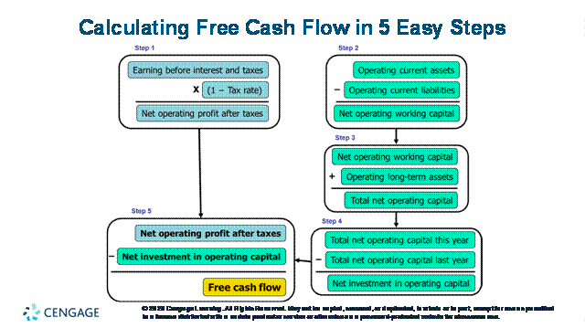
a Free account - it's easy! 5. Follow the instructions and start trading! Chapter 2 Financial
Statements Topics in Chapter 2: ·
Introduction
of Financial Statement ·
Firm’s
Intrinsic Value ·
Balance
Sheet ·
Income
Statement ·
Cash
Flow Statement ·
Free
Cash Flow
|
||||||||||||||||||||||||||||||||||||||||||||||||||||||||||||||||||||||||||||||||||||||||||||||||||||||||||||||||||||||||||||||||||||||||||||||||||||||||||||||||||||||||||||||||||||||||||||||||||||||||||||||||||||||||||||||||||||||||||||||||||||||||||||||||||||||||||||||||||||||||||||||||||||||||||||||||||||||||||||||||||||||||||||||||||||||||||||||||||||||||||||||||||||||||||||||||||||||||||||||||||||||||||||||||||||||||||||||||||||||||||||||||||||||||||||||||||||||||||||||||||||||||||||||||||||||||||||||||||||||||||||||||||||||||||||||||||||||||||||||||||||||||||||||||||||||||||||||||||||||||||||||||||||||||||||||||||||||||||||||||||||||||||||||||||||||||||||||||||||||||||||||||||||||||||||||||||||||||||||||||||||||||||||||||||||||||||||||||||||||||||||||||||||||||||||||||||||||||||||||||||||||||||||||||||||||||||||||||||||||||||||||||||||||||||||||||||||||||||||||||||||||||||||||||||||||||||||||||||||||||||||||||||||||||||||||||||||||||||||||||||||||||||||||||||||||||||||||||||||||
|
||
|
Amount |
||
|
Sales |
$785 |
|
|
Total cost of goods sold |
$460 |
|
|
Gross profit (EBITDA) |
$325 |
|
|
Depreciation |
$210 |
|
|
Operating expenses |
$0 |
|
|
Operating income (EBIT) |
$115 |
|
|
Interest expenses |
$35 |
|
|
Taxable income (EBT) |
$80 |
|
|
Taxes on income |
$28 |
|
|
Net income |
$52 |
• What is the cash flow from investment for 2015? ($57)
• What is the cash flow from operating for 2015? ($360)
• What is the cash flow from financing for 2015? ($-412)
Answer: https://www.jufinance.com/10k/cf/
|
Cash Flow Statement Template |
|
|
Cash at the beginning of the
year |
70 |
|
Cash
from operation |
|
|
net income |
52 |
|
plus depreciation |
210 |
|
-/+ AR |
61 |
|
-/+
Inventory |
22 |
|
+/- AP |
15 |
|
net
change in cash from operation |
360 |
|
Cash
from investment |
|
|
-/+ (NFA+depreciation) |
57 |
|
net
change in cash from investment |
57 |
|
Cash
from financing |
|
|
+/- long term debt |
70 |
|
+/- common stock |
-465 |
|
- dividend |
-17 |
|
net
change in cash from investment |
-412 |
|
Total
net change of cash |
5 |
|
Cash
at the end of the year |
75 |
Chapter 3 Analysis
of Financial Statements
Topics in Chapter 3:
1.
Ratio
analysis
2.
DuPont
equation
3.
Benchmarking
for ratio analysis
4.
Limitations
of ratio analysis
5.
Qualitative
factors
Ratio Analysis template
https://www.jufinance.com/ratio
Finviz.com/screener for ratio
analysis (https://finviz.com/screener.ashx
Financial ratio analysis (VIDEO)
****** DuPont Identity
*************
ROE = (net income / sales) *
(sales / assets) * (assets / shareholders' equity)
This equation for ROE breaks it
into three widely used and studied components:
ROE = (net profit margin) * (asset
turnover) * (equity multiplie)
In
class exercise
Firm AAA’s total asset = $720,000. This company has no debt, so its debt/equity ratio = 0%. Now the CEO wants to raise the debt/assets ratio to 40%. How much must the firm borrow to achieve this goal?
a. $273,600
b. $288,000
c. $302,400
d. $327,100
answer: Total assets $720,000
Target debt ratio 40%
Debt to achieve target ratio = Amount borrowed = Target % × Assets = $288,000
Week 1 case study – chapters 2 and 3 (due by 6/5/2021)
Help video url: https://www.jufinance.com/video/fin534_case1_2021_spring.mp4 -- posted
How much does Amazon worth?” --- FYI only: Amazon.com Inc. (AMZN) https://www.stock-analysis-on.net/NASDAQ/Company/Amazoncom-Inc/DCF/Present-Value-of-FCFF
Present
Value of Free Cash Flow to the Firm (FCFF)
In
discounted cash flow (DCF) valuation techniques the value of the stock is
estimated based upon present value of some measure of cash flow. Free cash
flow to the firm (FCFF) is generally described as cash flows after direct
costs and before any payments to capital suppliers.
- Intrinsic Stock Value
(Valuation Summary)
- Weighted Average Cost of
Capital (WACC)
- FCFF Growth Rate (g)
Intrinsic Stock Value (Valuation Summary)
Amazon.com
Inc., free cash flow to the firm (FCFF) forecast
|
Year |
Value |
FCFFt or Terminal value (TVt) |
Calculation |
Present
value at 16.17% |
|
01 |
FCFF0 |
(4,286) |
||
|
1 |
FCFF1 |
– |
= (4,286) ×
(1 + 0.00%) |
– |
|
2 |
FCFF2 |
– |
= – ×
(1 + 0.00%) |
– |
|
3 |
FCFF3 |
– |
= – ×
(1 + 0.00%) |
– |
|
4 |
FCFF4 |
– |
= – ×
(1 + 0.00%) |
– |
|
5 |
FCFF5 |
– |
= – ×
(1 + 0.00%) |
– |
|
5 |
Terminal value (TV5) |
– |
= – ×
(1 + 0.00%) ÷ (16.17%
– 0.00%) |
– |
|
Intrinsic value of Amazon.com's capital |
– |
|||
|
Less: Debt (fair value) |
45,696 |
|||
|
Intrinsic value of Amazon.com's common stock |
– |
|||
|
Intrinsic value of Amazon.com's common stock (per share) |
$– |
|||
|
Current share price |
$1,642.81 |
|||
1
Weighted Average Cost of Capital (WACC)
Amazon.com
Inc., cost of capital
|
Value1 |
Weight |
Required
rate of return2 |
Calculation |
|
|
Equity (fair value) |
803,283 |
0.95 |
16.97% |
|
|
Debt (fair value) |
45,696 |
0.05 |
2.10% |
= 2.99%
× (1 – 29.84%) |
1 USD $ in millions
Equity (fair value) = No. shares
of common stock outstanding × Current share price
= 488,968,628 × $1,642.81 =
$803,282,551,764.68
Debt (fair value). See Details »
2 Required rate of return on equity
is estimated by using CAPM. See Details »
Required rate of return on debt. See Details »
Required rate of return on debt
is after tax.
Estimated (average) effective
income tax rate
= (20.20% + 36.61%
+ 60.59% + 0.00%
+ 31.80%) ÷ 5 = 29.84%
WACC
= 16.17%
FCFF Growth Rate (g)
FCFF growth rate
(g) implied by PRAT model
Amazon.com
Inc., PRAT model
|
Average |
Dec
31, 2017 |
Dec
31, 2016 |
Dec
31, 2015 |
Dec
31, 2014 |
Dec
31, 2013 |
||
|
Selected
Financial Data (USD $ in millions) |
|||||||
|
Interest expense |
848 |
484 |
459 |
210 |
141 |
||
|
Net income (loss) |
3,033 |
2,371 |
596 |
(241) |
274 |
||
|
Effective income tax rate
(EITR)1 |
20.20% |
36.61% |
60.59% |
0.00% |
31.80% |
||
|
Interest expense, after tax2 |
677 |
307 |
181 |
210 |
96 |
||
|
Interest expense (after tax)
and dividends |
677 |
307 |
181 |
210 |
96 |
||
|
EBIT(1 – EITR)3 |
3,710 |
2,678 |
777 |
(31) |
370 |
||
|
Current portion of long-term
debt |
100 |
1,056 |
238 |
1,520 |
753 |
||
|
Current portion of capital
lease obligation |
5,839 |
3,997 |
3,027 |
2,013 |
955 |
||
|
Current portion of finance
lease obligations |
282 |
144 |
99 |
67 |
28 |
||
|
Long-term debt, excluding
current portion |
24,743 |
7,694 |
8,235 |
8,265 |
3,191 |
||
|
Long-term capital lease
obligations, excluding current portion |
8,438 |
5,080 |
4,212 |
3,026 |
1,435 |
||
|
Long-term finance lease
obligations, excluding current portion |
4,745 |
2,439 |
1,736 |
1,198 |
555 |
||
|
Total stockholders' equity |
27,709 |
19,285 |
13,384 |
10,741 |
9,746 |
||
|
Total capital |
71,856 |
39,695 |
30,931 |
26,830 |
16,663 |
||
|
Ratios |
|||||||
|
Retention rate (RR)4 |
0.82 |
0.89 |
0.77 |
– |
0.74 |
||
|
Return on invested capital
(ROIC)5 |
5.16% |
6.75% |
2.51% |
-0.12% |
2.22% |
||
|
Averages |
|||||||
|
RR |
0.80 |
||||||
|
ROIC |
3.31% |
||||||
|
Growth rate of FCFF (g)6 |
0.00% |
||||||
2017
Calculations
2 Interest expense, after tax =
Interest expense × (1 – EITR)
= 848 × (1 – 20.20%)
= 677
3 EBIT(1 – EITR) = Net income
(loss) + Interest expense, after tax
= 3,033 + 677 = 3,710
4 RR = [EBIT(1 – EITR) – Interest
expense (after tax) and dividends] ÷ EBIT(1 – EITR)
= [3,710 – 677]
÷ 3,710 = 0.82
5 ROIC = 100 × EBIT(1 – EITR) ÷
Total capital
= 100 × 3,710 ÷ 71,856 = 5.16%
6 g = RR × ROIC
= 0.80 × 3.31%
= 0.00%
FCFF growth rate
(g) forecast
Amazon.com
Inc., H-model
|
Year |
Value |
gt |
|
1 |
g1 |
0.00% |
|
2 |
g2 |
0.00% |
|
3 |
g3 |
0.00% |
|
4 |
g4 |
0.00% |
|
5 and thereafter |
g5 |
0.00% |
where:
g1 is implied by PRAT model
g5 is implied by single-stage model
g2, g3 and g4 are calculated using linear interpoltion between g1 and g5
Calculations
g2 = g1 + (g5 – g1) × (2 – 1) ÷ (5 – 1)
= 0.00% + (0.00%
– 0.00%) × (2 – 1) ÷ (5 – 1) = 0.00%
g3 = g1 + (g5 – g1) × (3 – 1) ÷ (5 – 1)
= 0.00% + (0.00%
– 0.00%) × (3 – 1) ÷ (5 – 1) = 0.00%
g4 = g1 + (g5 – g1) × (4 – 1) ÷ (5 – 1)
= 0.00% + (0.00%
– 0.00%) × (4 – 1) ÷ (5 – 1) = 0.00%
6/5 -1
Chapter 1 An
Overview of Financial Management
Chapter overview:
This chapter provides a basic idea of what financial
management/managerial finance/corporate finance is all about, including an
overview of the financial environment (financial markets, institutions, and
securities/instruments) in which
corporations operate.
Note:
Flow of funds describes the
financial assets flowing from various sectors through financial
intermediaries for the purpose of buying physical or financial assets.
*** Household, non-financial business,
and our government
Financial institutions facilitate
exchanges of funds and financial products.
*** Building blocks of a financial
system. Passing and transforming funds and risks during transactions.
*** Buy and sell, receive and
deliver, and create and underwrite financial products.
*** The transferring of funds and
risk is thus created. Capital utilization for individual and for the whole
economy is thus enhanced.
Negative interest rate
How
do negative interest rates work? | CNBC Explains
Chapter 4 Time
Value of Money
(review)
Topics:
·
Future Value and Compounding
·
Present Value and Discounting
·
Rates of Return/Interest Rates
·
Number of periods
·
Amortization
Amortization Table example:
- Develop an amortization
schedule in Excel for a five-year car loan of $30,000 with APR of 3%
(use the home mortgage loan as an example)
Hint: In excel, find amortization
template.
Calculator:
https://www.jufinance.com/tvm/
--- TVM calculator
https://www.jufinance.com/nfv/ --- net future value calculator
Equations:
FV = PV *(1+r)^n
PV = FV / ((1+r)^n)
N = ln(FV/PV) / ln(1+r)
Rate = (FV/PV)1/n -1
Annuity:
N
= ln(FV/C*r+1)/(ln(1+r))
Or
N = ln(1/(1-(PV/C)*r)))/
(ln(1+r))
Excel
Formulas
To get FV, use FV
function.
=abs(fv(rate, nper, pmt, pv))
To get PV, use PV
function
= abs(pv(rate, nper, pmt, fv))
To get r, use rate function
= rate(nper, pmt, pv, -fv)
To get number of years,
use nper function
= nper(rate, pmt, pv,
-fv)
To get annuity payment, use PMT
function
= abs(pmt(rate, nper, pv,
-fv))
In Class Exercise:
1. You want to retire early
so you know you must start saving money. Thus, you have decided to save
$4,500 a year, starting at age 25. You plan to retire as soon as you can
accumulate $500,000. If you can earn an average of 11 percent on your
savings, how old will you be when you retire? (49.74 years)
Answer: nper(11%, 4500, 0,
-500000)+25
2. Fred was persuaded to open a credit card account and now owes $5,150
on this card. Fred is not charging any additional purchases because he wants
to get this debt paid in full. The card has an APR of 15.1 percent. How much
longer will it take Fred to pay off this balance if he makes monthly payments
of $70 rather than $85? (93.04 months)
Answer: nper(15.1%/12, 70, -5150,
0) - nper(15.1%/12, 85, -5150, 0)
3. At the end of this month, Bryan will start saving $80 a month for
retirement through his company's retirement plan. His employer will
contribute an additional $.25 for every $1.00 that Bryan saves. If he is
employed by this firm for 25 more years and earns an average of 11 percent on
his retirement savings, how much will Bryan have in his retirement account 25
years from now? ($157,613.33)
Answer: Bryan’s monthly contribution: 80+80*0.25 = 100
Fv(11%/12, 25*12, 100, 0))
4. Sky Investments offers an
annuity due with semi-annual payments for 10 years at 7 percent interest. The
annuity costs $90,000 today. What is the amount of each annuity
payment? ($6,118.35)
Answer: pmt(7%/2, 10*2, 90000,
0,1)
5. Mr. Jones just won a lottery prize that will pay him $5,000 a year
for thirty years. If Mr. Jones can
earn 5.5 percent on his money, what are his
winnings worth to him today? ($72,668.73)
Answer: pv(5.5%, 30, 5000, 0)
Chapter 5 Bond,
Bond Valuation and Interest Rates
Topics in Chapter 5:
·
Key features of bonds
·
Bond valuation
·
Measuring yield
·
Assessing risk
Market data website:
1. FINRA
http://finra-markets.morningstar.com/BondCenter/Default.jsp (FINRA
bond market data)
2. WSJ
Market watch on Wall Street Journal has daily yield curve
and bond yield information.
http://www.marketwatch.com/tools/pftools/
https://www.youtube.com/watch?v=yph8TRldW6k
3. Bond Online
http://www.bondsonline.com/Todays_Market/
Simplified Balance
Sheet of WalMart
|
In Millions of USD |
As of 2020-01-31 |
|
Total Assets |
236,495,000 |
|
Total Current
Liabilities |
16,203,000 |
|
Long Term Debt |
64,192,000 |
|
Total Liabilities |
154,943,000 |
|
Total Equity |
81,552,000 |
|
Total Liabilities
& Shareholders' Equity |
236,495,000 |
https://www.wsj.com/market-data/quotes/WMT/financials/annual/balance-sheet
FINRA – Bond market
information
http://finra-markets.morningstar.com/BondCenter/Default.jsp
WAL-MART
STORES INC
http://finra-markets.morningstar.com/BondCenter/BondDetail.jsp?ticker=C104227&symbol=WMT.GP
Coupon
Rate
7.550
%
Maturity
Date
02/15/2030
Symbol
WMT.GP |
CUSIP
931142BF9 |
Next Call Date
— |
Callable
— |
Last Trade Price
$146.28 |
Last Trade Yield
1.776% |
Last Trade Date
06/04/2021 |
US Treasury Yield
— |
|
|
Credit
and Rating Elements
|
Moody's® Rating |
Aa2 (5/9//2018) |
|
Standard & Poor's
Rating |
AA (02/10/2000) |
|
TRACE Grade |
Investment Grade |
|
Default |
— |
|
Bankruptcy |
N |
|
Insurance |
— |
|
Mortgage Insurer |
— |
|
Pre-Refunded/Escrowed |
— |
|
Additional Description |
Senior Unsecured Note |
Classification Elements
|
Bond Type |
US Corporate Debentures |
|
Debt Type |
Senior Unsecured Note |
|
Industry Group |
Industrial |
|
Industry Sub Group |
Retail |
|
Sub-Product Asset |
CORP |
|
Sub-Product Asset Type |
Corporate Bond |
|
State |
— |
|
Use of Proceeds |
— |
|
Security Code |
— |
Special
Characteristics
|
Medium Term Note |
N |
Issue Elements
|
*dollar
amount in thousands |
|
|
Offering Date |
02/09/2000 |
|
Dated Date |
02/15/2000 |
|
First Coupon Date |
08/15/2000 |
|
Original Offering* |
$1,000,000.00 |
|
Amount Outstanding* |
$1,000,000.00 |
|
Series |
— |
|
Issue Description |
— |
|
Project Name |
— |
|
Payment Frequency |
Semi-Annual |
|
Day Count |
30/360 |
|
Form |
Book Entry |
|
Depository/Registration |
Depository Trust Company |
|
Security Level |
Senior |
|
Collateral Pledge |
— |
|
Capital Purpose |
— |
Bond Elements
|
*dollar
amount in thousands |
|
|
Original Maturity Size* |
1,000,000.00 |
|
Amount Outstanding Size* |
1,000,000.00 |
|
Yield at Offering |
7.56% |
|
Price at Offering |
$99.84 |
|
Coupon Type |
Fixed |
|
Escrow Type
|
|
·
The attached Wal-mart Bond prospects says:
“We are offering $500,000,000 of our 1.000% notes due 2017 (symbol WMT4117476),
$1,000,000,000 of our 3.300% notes due 2024 (symbol WMT4117477) and
$1,000,000,000 of our 4.300% notes due 2044 (symbol WMT4117478)
Risk of Bonds
Class discussion: Is bond market risky?
Bond
risk (video)
Bond
risk – credit risk (video)
Bond
risk – interest rate risk (video)
Bond
risk – how to reduce your risk (video)
1. AAA
firm’s bonds’ market value is
$1,120, with 15 years maturity and coupon of $85. What is YTM? (7.17%, rate(15, 85, -1120, 1000))
2. Sadik
Inc.'s bonds currently sell for $1,180 and have a par value of
$1,000. They pay a $105 annual coupon
and have a 15-year maturity, but they can be called in 5 years at
$1,100. What is their yield to call (YTC)? (7.74%, rate(5, 105, -1180, 1100))
3. Assume
that you are considering the purchase of a 20-year, noncallable bond with an
annual coupon rate of 9.5%. The bond has a face value of $1,000,
and it makes semiannual interest payments. If you require an 8.4%
nominal yield to maturity on this investment, what is the maximum price you
should be willing to pay for the bond? ($1,105.69, abs(pv(8.4%/2,
20*2, 9.5%*1000/2, 1000)) )
4. McCue
Inc.'s bonds currently sell for $1,250. They pay a $90 annual coupon, have a
25-year maturity, and a $1,000 par value, but they can be called in 5 years
at $1,050. Assume that no costs other than the call premium would
be incurred to call and refund the bonds, and also assume that the yield curve is horizontal, with
rates expected to remain at current levels on into the
future. What is the difference between this bond's YTM and its
YTC? (Subtract the YTC from the YTM; it is possible to get a
negative answer.) (2.62%, YTM = rate(25, 90, -1250, 1000), YTC = rate(5, 90, -1250, 1050))
5. A
25-year, $1,000 par value bond has an 8.5% annual payment
coupon. The bond currently sells for $925. If the yield
to maturity remains at its current rate, what will the price be 5 years from
now? ($930.11, rate(25, 85, -925, 1000), abs(pv( rate(25, 85, -925, 1000),
20, 85, 1000))
Assignments
(due with the mid-term exam)
part 1 (help video: https://www.jufinance.com/video/fin534_case2_2021_spring_part_1.mp4) – posted
part 2 (help video: https://www.jufinance.com/video/fin534_case2_2021_spring_part_2.mp4) – posted
2.
Develop an amortization schedule in
Excel for a five-year car loan of $30,000 with APR of 3%
(hint: use amortization loan template
in excel)
3.
Chapter 4 End of Chapter Problems
(not questions): 1, 2, 3, 4, 16, 17, 19, 27 (chapter 4 homework solution all inclusive fyi only)
Chapter 4 Homework assignments – Spring 2021
Page 186:
4-1: If you deposit $10,000 in a bank account that pays 10% interest annually. How much will be in your account after 5 years?
4-2: What is the present value of a security that will pay $5000 in 20 years if securities of equal risk pay 7% annually.
4-3: Your parents will retire in 18 years. They currently have $250,000 and they think they will need $1 million at retirement. What annual interest rate must they earn to reach their goal, assuming they do not save any additional funds?
4-4: If you deposit money today in an account that pays 6.5% annual interest, how long will it take to double your money?
4-16: Find the amount to which $500 will grow under each of the following conditions.
a. 12% compounded annually for 5 years.
b. 12% compounded semiannually for 5 years.
c. 12% compounded quarterly for 5 years.
d. 12% compounded monthly for 5 years.
4-17: Find the present value of $500 due in the future under each of the following conditions.
a. 12% nominal rate, semiannual compounding, discounted back 5 years
b. 12% nominal rate, quarterly compounding, discounted back 5 years
c. 12% nominal rate, monthly compounding, discounted back 5 years
4-19: Universal bank
pays 7% interest, compounded annually, on time deposits. Regional
bank pays 6% interest, compounded quarterly.
a.
Based on effective interest rates, in
which bank would you prefer to deposit your money?
b.
Could your choice of banks be influenced
by the fact that you might want o withdraw your funds during the year as
opposed to at the end of the year? In answering this question, assume that
funds must be left on deposit during an entire compounding period in order
for you to receive any interest.
4-27:
What is the present value of a perpetuity of $100
per year if the appropriate discount rate is 7%? If interest rates in general
were to double and the appropriate discount rate rose to 14%, what would
happen to the present value of the perpetuity?
Updated
Feb 26, 2021
What Are Negative Interest Rates? (FYI)
Negative
interest rates occur when borrowers are credited interest rather than paying
interest to lenders. While this is a very unusual scenario, it is most likely
to occur during a deep economic recession when monetary efforts and market
forces have already pushed interest rates to their nominal zero bound.
Typically,
a central bank will charge commercial banks on their reserves as a form of
non-traditional expansionary monetary policy, rather than crediting them interest.
This extraordinary monetary policy tool is used to strongly encourage
lending, spending, and investment rather than hoarding cash, which will lose
value to negative deposit rates. Note that individual depositors will not be
charged negative interest rates on their bank accounts.
KEY
TAKEAWAYS
• Negative interest rates occur when
borrowers are credited interest rather than paying interest to lenders.
• With negative interest rates,
central banks charge commercial banks on reserves in an effort to incentivize
them to spend rather than hoard cash positions.
• With negative interest rates,
commercial banks are charged interest to keep cash with a nation's central
bank, rather than receiving interest. Theoretically, this dynamic should
trickle down to consumers and businesses, but commercial banks have been
reluctant to pass negative rates onto their customers.
Understanding
a Negative Interest Rate
While
real interest rates can be effectively negative if inflation exceeds the
nominal interest rate, the nominal interest rate is, theoretically, bounded
by zero. Negative interest rates are often the result of a desperate and
critical effort to boost economic growth through financial means.
The
zero-bound refers to the lowest level that interest rates can fall to; some
forms of logic would dictate that zero would be that lowest level. However,
there are instances where negative rates have been implemented during normal
times. Switzerland is one such example; as of mid-2020, its target interest
rate was -0.75%.1 Japan adopted a similar policy, with a mid-2020 target rate
of -0.1%.2
Negative
interest rates may occur during deflationary periods. During these times,
people and businesses hold too much money—instead of
spending money—with the expectation that a dollar
will be worth more tomorrow than today (i.e., the opposite of inflation).
This can result in a sharp decline in demand, and send prices even lower.
Often,
a loose monetary policy is used to deal with this type of situation. However,
when there are strong signs of deflation factoring into the equation, simply
cutting the central bank's interest rate to zero may not be sufficient enough
to stimulate growth in both credit and lending.
In a
negative interest rate environment, an entire economic zone can be impacted
because the nominal interest rate dips below zero. Banks and financial firms
have to pay to store their funds at the central bank, rather than earn
interest income.
Consequences
of Negative Rates
A
negative interest rate environment occurs when the nominal interest rate
drops below zero percent for a specific economic zone. This effectively means
that banks and other financial firms have to pay to keep their excess
reserves stored at the central bank, rather than receiving positive interest income.
A
negative interest rate policy (NIRP) is an unusual monetary policy tool.
Nominal target interest rates are set with a negative value, which is below
the theoretical lower bound of zero percent.
During
deflationary periods, people and businesses tend to hoard money, instead of
spending money and investing. The result is a collapse in aggregate demand,
which leads to prices falling even further, a slowdown or halt in real
production and output, and an increase in unemployment.
A loose
or expansionary monetary policy is usually employed to deal with such
economic stagnation. However, if deflationary forces are strong enough,
simply cutting the central bank's interest rate to zero may not be sufficient
to stimulate borrowing and lending.
Example
of a Negative Interest Rate
In
recent years, central banks in Europe, Scandinavia, and Japan have
implemented a negative interest rate policy (NIRP) on excess bank reserves in
the financial system. This unorthodox monetary policy tool is designed to
spur economic growth through spending and investment; depositors would be
incentivized to spend cash rather than store it at the bank and incur a
guaranteed loss.
It's
still not clear if this policy has been effective in achieving this goal in
those countries, and in the way it was intended. It's also unclear whether or
not negative rates have successfully spread beyond excess cash reserves in
the banking system to other parts of the economy.
Frequently
Asked Questions
How can
interest rates turn negative?
Interest
rates tell you how valuable money is today compared to the same amount of
money in the future. Positive interest rates imply that there is a time value
of money, where money today is worth more than money tomorrow. Forces like
inflation, economic growth, and investment spending all contribute to this
outlook. A negative interest rate, by contrast, implies that your money will
be worth more in the future, not less.
What do negative interest rates mean for
people?
Most instances of negative interest rates
only apply to bank reserves held by central banks; however, we can ponder the
consequences of more widespread negative rates. First, savers would have to
pay interest instead of receiving it. By the same token, borrowers would be
paid to do so instead of paying their lender. Therefore, it would incentivize
many to borrow more and larger sums of money and to forgo saving in favor of
consumption or investment. If they did save, they would save their cash in a
safe or under the mattress, rather than pay interest to a bank for depositing
it. Note that interest rates in the real world are set by the supply and
demand for loans (despite central banks setting a target). As a result, the
demand for money in-use would grow and quickly restore a positive interest
rate.
Where
do negative interest rates exist?
Some
central banks have set a negative interest rate policy (NIRP) in order to
stimulate economic growth in the financial sector, or else to protect the
value of a local currency against exchange-rate increases due to large
inflows of foreign investment. Countries including Japan, Switzerland,
Sweden, and even the ECB (eurozone) have adopted NIRPs at various points over
the past two decades.
Why
would a central bank adopt a NIRP to stimulate the economy?
Monetary
policymakers are often afraid of falling into a deflationary spiral. In harsh
economic times, such as deep economic recessions or depressions, people and
businesses tend to hold on to their cash while they wait for the economy to
improve. This behavior, however, can weaken the economy further as a lack of
spending causes further job losses, lowers profits, and prices to drop—all of which reinforces people’s
fears, giving them even more incentive to hoard. As spending slows even more,
prices drop again, creating another incentive for people to wait as prices
fall further. And so on. When central banks have already lowered interest
rates to zero, the NIRP is a way to incentivize corporate borrowing and
investment and discourage hoarding of cash.
https://www.investopedia.com/terms/n/negative-interest-rate.asp
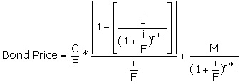
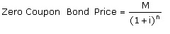
Bond Pricing Formula (FYI)
![]()
Bond Pricing Excel Formula
To calculate bond
price in EXCEL (annual coupon bond):
Price=abs(pv(yield to maturity, years
left to maturity, coupon rate*1000, 1000)
To calculate yield
to maturity (annual coupon bond)::
Yield to maturity = rate(years left to
maturity, coupon rate *1000, -price, 1000)
To calculate bond
price (semi-annual coupon bond):
Price=abs(pv(yield to maturity/2,
years left to maturity*2, coupon rate*1000/2, 1000)
To calculate yield
to maturity (semi-annual coupon bond):
Yield to maturity = rate(years left to
maturity*2, coupon rate *1000/2, -price, 1000)*2
Function Description
The Excel Price
function calculates the price, per $100 face value of a security that pays
periodic interest.
The syntax of the
function is:
PRICE( settlement, maturity, rate, yld, redemption, frequency, [basis] )
The Excel YIELD
function calculates the Yield of a security that pays periodic interest.
The syntax of the
function is:
YIELD( settlement, maturity, rate, pr, redemption, frequency, [basis] )
Where the arguments
are as follows:
|
pr |
- |
The security's price
per $100 face value. |
|
settlement |
- |
The settlement date of
the security (i.e. the date that the coupon is purchased). |
||||||||||||
|
maturity |
- |
The maturity date of
the security (i.e. the date that the coupon expires). |
||||||||||||
|
Rate |
- |
The security's
annual coupon rate. |
||||||||||||
|
Yld |
- |
The annual yield of
the security. |
||||||||||||
|
redemption |
- |
The security's
redemption value per $100 face value. |
||||||||||||
|
frequency |
- |
The number of coupon payments per year. This
must be one of the following:
|
||||||||||||
|
[basis] |
- |
An optional integer
argument which specifies the financial day count basis that is used by the
security. Possible values are: |
||||||||||||
|
||||||||||||||
|
The financial day
count basis rules are explained in detail on the Wikipedia Day Count
Convention page |
||||||||||||||
https://www.excelfunctions.net/excel-price-function.html
https://www.excelfunctions.net/excel-yield-function.html
Function Description
The Excel Accrint
function returns the accrued interest for a security that pays periodic
interest.
The syntax of the
function is:
ACCRINT( issue, first_interest, settlement, rate, [par], frequency, [basis], [calc_method] )
Where the arguments
are as follows:
|
issue |
- |
The issue date of
the security. |
|
first_interest |
- |
The security's first
interest date. |
|
settlement |
- |
The security's
settlement date. |
|
rate |
- |
The security's
annual coupon rate. |
|
[par] |
- |
The security's par value. If omitted, [par] takes the
default value of 1,000. |
|
frequency |
- |
The number of coupon
payments per year (must be equal to 1, 2 or 4). |
|
[basis] |
- |
An optional argument, that specifies the day
count basis to be used in the calculation. |
|
|
Chapter 6 Risk
and Return
Topics in Chapter 6:
·
Basic return and risk concepts
·
Stand-alone risk
·
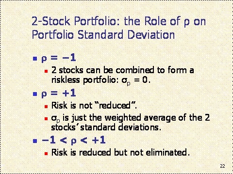
Risk in a Portfolio Context
·
Risk and return: CAPM/SML
·
Market equilibrium and market efficiency
Please use the
following Excel file to learn how to estimate how risky those securities are.
WMT,
Tesla, Apple, and S&P500 stock prices April 2016 ~ May 2021
(solution. Updated for S&P on 6/4/2021)
Summary of Excel
functions:
Mean --- average
function
Risk (standard
deviation) --- stdev function
Correlation between
two stocks --- correl function
Covariance between two
stocks --- covar function
Beta (risk) --- slope
function
A Single Stock, like WMT
Example:
1. Realized return
Holding period return (HPR) = (Selling price – Purchasing price
+ dividend)/ Purchasing price
HPR calculator (www.jufinance.com/hpr)
2. Expected return of this stock and its standard
deviation
Expected return and risk
(standard deviation) calculator (www.jufinance.com/return)
A portfolio of two stocks, like WMT and Amazon
Portfolio Calculator (www.jufinance.com/portfolio) – see equations
below
Equation:
![]()
W1 and W2 are the
percentage of each stock in the portfolio.
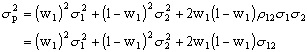
![]()
- σ12 = the correlation
coefficient between the returns on stocks 1 and 2,
- Cov12 = the
covariance between the returns on stocks 1 and 2,
- σ1 = the standard
deviation on stock 1, and
- σ2 = the standard
deviation on stock 2.
![]()
- σ12 = the covariance
between the returns on stocks 1 and 2,
- N = the number of states,
- pi = the
probability of state i,
- R1i = the
return on stock 1 in state i,
- E[R1] = the
expected return on stock 1,
- R2i = the
return on stock 2 in state i, and
- E[R2] = the
expected return on stock 2.
A portfolio of three stocks, like WMT, Amazon, and APPLE
Three stocks is the
sum of three pairs of two-stock-portfolio. So same as above but repeat it
three times.
A diversified portfolio with 25 stocks and more
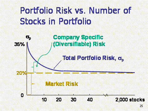
As more stocks are
added, each new stock has a smaller risk-reducing impact on the portfolio.
sp falls very slowly after about
40 stocks are included. The lower limit for sp is
about 20% = sM (M: market portfolio).
By forming well-diversified portfolios,
investors can eliminate about half the risk of owning a single stock.
Market risk is that part of a security’s stand-alone
risk that cannot be eliminated by diversification.
Firm-specific, or diversifiable, risk is that
part of a security’s stand-alone risk that can be eliminated by
diversification.
CAPM model (CAPM calculator)
1. What is Beta? Where to find Beta?

2. Why can we use beta as measure for risk?
3. What is three month Treasurye bill’s beta?
S&P500 index’s beta? WMT’s beta? Amazon’s beta? Why are they different?
4. Use CAPM to calculate the expected return of
the above stocks
5. Find those stocks in SML
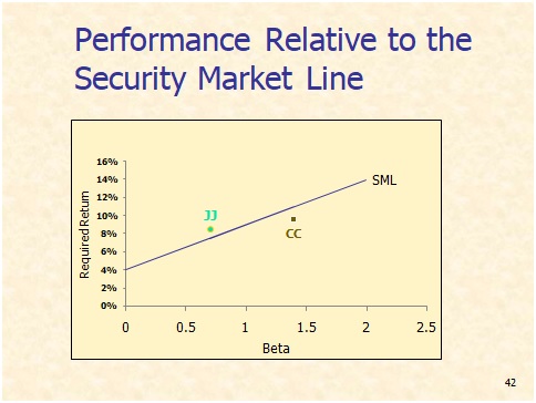
6. What is market efficiency? Do you agree with the
hypothesis that market is efficient? Do you have any evidence to disapprove
it? What Is the Efficient
Market Hypothesis? (youtube)
Assignment of chapter
6: Chapter 6 Case study (due with mid term exam)
(help video: https://www.jufinance.com/video/fin534_case3_2021_spring.mp4)
No other problem solving assignments for
chapter 6
How do you compute the Beta of a company
First, we need to have two samples of the
same size: The returns for a company, and the returns of the market
for the same period of time. Note: You need to provide
the returns and NOT the actual stock values in order for the calculations to
be correct.
Then, a linear regression is conducted
and the estimated slope of the regression model using the returns of the
company as the dependent variable and the returns of the market as the
independent variable will be the beta we are looking for.
Alternative
formulas to compute the beta https://mathcracker.com/beta-calculator
The actual definition of beta is :
This formula is less clear for many people
because the covariance is a less understood
measure and some people do not know how to compute it.
Ultimately, the calculation
of the beta as a slope coefficient of the regression between company and
market returns has a stronger intuitive appeal.
Beta Calculator Excel
Calculation beta in Excel is easy. You need to go to a
provider of historical prices, such as Yahoo finance. Then you clean all
you need to clean and leave only adjusted prices.
Your market data could be
the S&P 500 or any other market proxy. Then, by subtracting and dividing
by the base value, you will get the returns, for both your company and the
market.
Then, you will run a
regression with the company returns as the dependent variable, and the market
returns as the independent variable.
Finally, you will examine
your regression output, and select the estimated slope coefficient. That will
be the beta you are looking for.
Beta calculator and the CAPM
Why is it useful to compute the beta of a firm? Because it
gives a measure of how risky the firm's stock is with respect to the market,
and it tells us how much should be our expected return based ion that level
of risk, via de CAPM model.
RISK and Return General Template (standard deviation, correlation, beta)
In Class
Exercise
1. An investor currently holds the following portfolio: He
invested 30% of the fund in Apple with Beta equal 1.1. He also invested 40%
in GE with Beta equal 1.6. The rest of his fund goes to Ford, with Beta equal
2.2. Use the above information to answer the following questions.
1) The beta for the portfolio is? (1.63)
2) The three month Treasury bill rate (this is
risk free rate) is 2%. S&P500 index return is 10% (this is market
return). Now calculate the portfolio’s return. (15.04%)
Answer:
1) Portfolio beta = 0.3*1.1 + 0.4*1.6 +
(1-0.3-0.4)*2.2 = 1.63
2)
Portfolio return
= 2% + 1.63*(10%-2%) = 15.04%
2. Your current portfolio’s
BETA is about 1.2. Your total investment is worth around $200,000. You uncle
just gave you $100,000 to invest for him. With this $100,000 extra funds in
hand, you plan to invest the whole $100,000 in additional stocks to increase
your whole portfolio’s BETA to 1.5 (Your portfolio now worth $200,000 plus
$100,000). What is the average BETA of the new stocks to achieve your goal?
(hint: write down the equation of the portfolio’s Beta first) (2.1)
Answer:
·
Weight of
the original fund = 200000/(200000+100000) = 2/3
·
Weight of
new fund = 1-2/3 = 1/3
·
So protfolio
beta = 1.5 = (2/3)*1.2 + (1/3)* X è X=2.1
3. What is the coefficient of variation on
the company's stock?
Probability Stock's
State
of of
State
the
Economy Return
Boom 0.45 25%
Normal 0.50 15%
Recession 0.05 5%
ANSWER:
Or,
Probability
of Return Deviation Squared State
Prob.
This
state This
state from
Mean Deviation ×
Sq. Dev.
0.45 25.00% 6.00% 0.36% 0.1620%
0.50 15.00% -4.00% 0.16% 0.0800%
0.05 5.00% -14.00% 1.96% 0.0980%
Expected return = 19.00% 0.34% 0.3400% =
Expected variance
σ
= 5.83%
Coefficient
of variation = σ/Expected return = 0.3069
4. What's the
standard deviation?
Economic
Conditions Prob. Return
Strong 30% 32.0%
Normal 40% 10.0%
Weak 30% -16.0%
ANSWER:
Or,
Economic Return Dev.
from Squared Sqd.
dev.
Conditions Prob. This
state Mean Dev. × Prob
Strong 30% 32.0% 23.20% 5.38% 1.61%
Normal 40% 10.0% 1.20% 0.01% 0.01%
Weak 30% -16.0% -24.80% 6.15% 1.85%
100% 8.8% Variance 3.47%
σ = Sqrt of
variance 18.62% 18.62% by
Excel
5. returns
are shown below. What's the standard deviation of the firm's
returns? (Hint: This is a sample, not a complete population.
USE the sample standard deviation formula)
Year Return
2008 21.00%
2007 -12.50%
2006 25.00%
ANSWER: IN
EXCEL, STDEV SYNTAX.
Or,
Deviation Squared
Year Return from
Mean Deviation
2008 21.00% 9.83% 0.97%
2007 -12.50% -23.67% 5.60%
2006 25.00% 13.83% 1.91%
Expected
return 11.17% 8.48% Sum
sqd deviations
4.24% Sum/(N
− 1)
SQRT = σ =
20.59% 20.59% with
Excel
Mid Term Exam (on blackboard, 6/11 –
6/20)
Review: https://www.jufinance.com/video/fin534_week4_2021_spring.mp4
Chapter 7 Valuation of Stocks and
Corporations
Topics in Chapter 7:
· Features
of common stock
· Valuing
common stock
o
Dividend growth model
o
Market multiples
· Preferred
stock
Part I: Dividends
For class discussion:
·
What
is dividend growth model? Why can we use dividend to estimate a firm’s
intrinsic value?
·
Are
future dividends predictable?
·
Refer
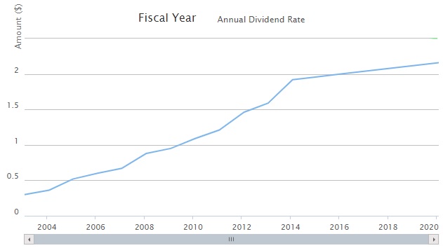
to the following table for WMT’s dividend history
http://stock.walmart.com/investors/stock-information/dividend-history/default.aspx
· Refer to the following table for Wal-mart (WMT’s dividend history)
http://stock.walmart.com/investors/stock-information/dividend-history/default.aspx
|
Record Dates |
Payable Dates |
Amount |
Type |
|
March 20, 2020 |
April 6, 2020 |
$0.54 |
Regular Cash |
|
May 8, 2020 |
June 1, 2020 |
$0.54 |
Regular Cash |
|
Aug. 14, 2020 |
Sept. 8, 2020 |
$0.54 |
Regular Cash |
|
Dec. 11, 2020 |
Jan. 4, 2021 |
$0.54 |
Regular Cash |
|
Record Dates |
Payable Dates |
Amount |
Type |
|
March 15, 2019 |
April 1, 2019 |
$0.53 |
Regular Cash |
|
May 10, 2019 |
June 3, 2019 |
$0.53 |
Regular Cash |
|
Aug. 9, 2019 |
Sept. 3, 2019 |
$0.53 |
Regular Cash |
|
Dec. 6, 2019 |
Jan. 2, 2020 |
$0.53 |
Regular Cash |
|
Record Dates |
Payable Dates |
Amount |
Type |
|
March 9, 2018 |
April 2, 2018 |
$0.52 |
Regular Cash |
|
May 11, 2018 |
June 4, 2018 |
$0.52 |
Regular Cash |
|
Aug. 10, 2018 |
Sept. 4, 2018 |
$0.52 |
Regular Cash |
|
Dec. 7, 2018 |
Jan. 2, 2019 |
$0.52 |
Regular Cash |
|
Record Dates |
Payable Dates |
Amount |
Type |
|
March 10, 2017 |
April 3, 2017 |
$0.51 |
Regular Cash |
|
May 12, 2017 |
June 5, 2017 |
$0.51 |
Regular Cash |
|
Aug. 11, 2017 |
Sept. 5, 2017 |
$0.51 |
Regular Cash |
|
Dec. 8, 2017 |
Jan. 2, 2018 |
$0.51 |
Regular Cash |
|
Record Dates |
Payable Dates |
Amount |
Type |
|
March 11, 2016 |
April 4, 2016 |
$0.50 |
Regular Cash |
|
May 13, 2016 |
June 6, 2016 |
$0.50 |
Regular Cash |
|
Aug. 12, 2016 |
Sep. 6, 2016 |
$0.50 |
Regular Cash |
|
Dec. 9, 2016 |
Jan. 3, 2017 |
$0.50 |
Regular Cash |
|
Record Dates |
Payable Dates |
Amount |
Type |
|
March 13, 2015 |
April 6, 2015 |
$0.490 |
Regular Cash |
|
May 8, 2015 |
June 1, 2015 |
$0.490 |
Regular Cash |
|
Aug. 7, 2015 |
Sep. 8, 2015 |
$0.490 |
Regular Cash |
|
Dec. 4, 2015 |
Jan. 4, 2016 |
$0.490 |
Regular Cash |
Stock Splits
Wal-Mart Stores, Inc. was incorporated on Oct. 31, 1969. On
Oct. 1, 1970, Walmart offered 300,000 shares of its common stock to the
public at a price of $16.50 per share. Since that time, we have had 11
two-for-one (2:1) stock splits. On a purchase of 100 shares at $16.50 per
share on our first offering, the number of shares has grown as follows:
|
2:1 Stock Splits |
Shares |
Cost per Share |
Market Price on Split Date |
Record Date |
Distributed |
|
On the Offering |
100 |
$16.50 |
|||
|
May 1971 |
200 |
$8.25 |
$47.00 |
5/19/71 |
6/11/71 |
|
March 1972 |
400 |
$4.125 |
$47.50 |
3/22/72 |
4/5/72 |
|
August 1975 |
800 |
$2.0625 |
$23.00 |
8/19/75 |
8/22/75 |
|
Nov. 1980 |
1,600 |
$1.03125 |
$50.00 |
11/25/80 |
12/16/80 |
|
June 1982 |
3,200 |
$0.515625 |
$49.875 |
6/21/82 |
7/9/82 |
|
June 1983 |
6,400 |
$0.257813 |
$81.625 |
6/20/83 |
7/8/83 |
|
Sept. 1985 |
12,800 |
$0.128906 |
$49.75 |
9/3/85 |
10/4/85 |
|
June 1987 |
25,600 |
$0.064453 |
$66.625 |
6/19/87 |
7/10/87 |
|
June 1990 |
51,200 |
$0.032227 |
$62.50 |
6/15/90 |
7/6/90 |
|
Feb. 1993 |
102,400 |
$0.016113 |
$63.625 |
2/2/93 |
2/25/93 |
|
March 1999 |
204,800 |
$0.008057 |
$89.75 |
3/19/99 |
4/19/99 |
Can you
estimate the expected dividend in 2022? And in 2023? And on and on…
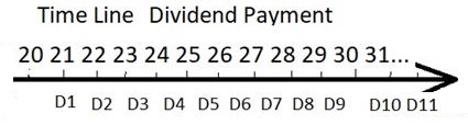
Can you write down the
math equation now?
WMT stock price = ?
Can you calculate now? It
is hard right because we assume dividend payment goes to infinity. How can we
simplify the calculation?
We can assume that
dividend grows at certain rate.
Discount rate is r (based
on Beta and CAPM that we have learned in chapter 6)
From finance.yahoo.com
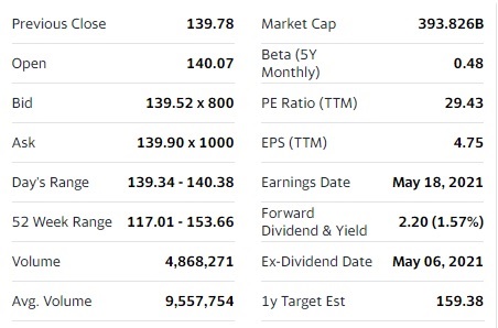
What does each item indicate?
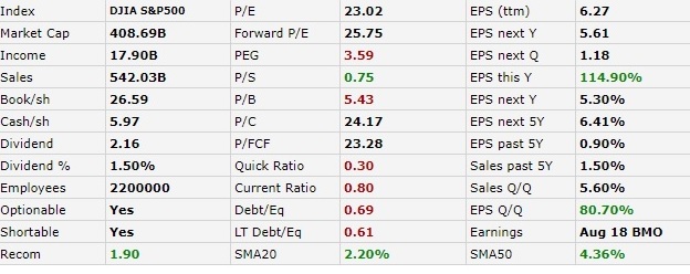
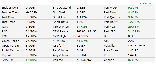
From finviz.com https://finviz.com/quote.ashx?t=WMT
Part II: Constant
Dividend Growth-Dividend growth model
Calculate stock prices
1) Given next dividends and price
Po= ![]()
Po= ![]() +
+![]()
Po= ![]() +
+![]() +
+![]()
Po= ![]() +
+![]() +
+![]() +
+![]()
……

Refer to http://www.calculatinginvestor.com/2011/05/18/gordon-growth-model/
· Now let’s apply this
Dividend growth model in problem solving.
Constant dividend growth
model calculator (www.jufinance.com/stock)
Equations
·
Po= D1/(r-g) or Po= Do*(1+g)/(r-g)
·
r = D1/Po+g = Do*(1+g)/Po+g
·
g= r-D1/Po = r- Do*(1+g)/Po
·
·
Capital Gain yield = g
·
·
Dividend Yield = r – g = D1 / Po = Do*(1+g) / Po
·
D1=Do*(1+g); D2= D1*(1+g);
D3=D2*(1+g)…
Exercise:
1.
Consider the
valuation of a common stock that paid $1.00 dividend at the end of the last
year and is expected to pay a cash dividend in the future. Dividends are
expected to grow at 10% and the investors required rate of return is 17%. How
much is the price? How much is the dividend yield? Capital gain yield?
2.
The current market
price of stock is $90 and the stock pays dividend of $3 with a growth rate of
5%. What is the return of this stock? How much is the dividend yield? Capital
gain yield?
Part III:
Non-Constant Dividend Growth
Calculate stock prices
1) Given next dividends and price
Po= ![]()
Po= ![]() +
+![]()
Po= ![]() +
+![]() +
+![]()
Po= ![]() +
+![]() +
+![]() +
+![]()
……
Non-constant dividend growth model calculator (https://www.jufinance.com/dcf/)
Equations
Pn = Dn+1/(r-g) = Dn*(1+g)/(r-g), since
year n, dividends start to grow at a constant rate.
Where Dn+1= next dividend in year n+1;
Do = just paid dividend in year n;
r=stock return; g= dividend growth rate;
Pn= current market price in year n;
Po = npv(r, D1, D2, …, Dn+Pn)
Or,
Po = D1/(1+r) + D2/(1+r)2 + … +
(Dn+Pn)/(1+r)n
In class exercise for non-constant dividend growth model
1. You
expect AAA Corporation to generate the following free cash flows over the
next five years:
|
Year |
1 |
2 |
3 |
4 |
5 |
|
FCF
($ millions) |
75 |
84 |
96 |
111 |
120 |
Since year
6, you estimate that AAA's free cash flows will grow at 6% per year. WACC of
AAA = 15%
·
Calculate the enterprise
value for DM Corporation.
·
Assume that AAA has $500
million debt and 14 million shares outstanding, calculate its stock price.
Answer:
|
FCF grows at 6% ==>
could use dividend constant growth model to get the value at year 5 |
|
Value in year five = FCF
in year 6 /(WACC - g) |
|
FCF in year 6 = FCF in
year 5 *(1+g%), g=6% |
|
FCF in year 6 = 120
*(1+6%) |
|
value in year five = 120*(1+6%)/(15%-6%)
= 1433.13 |
|
value in year 0 (current
value) =1017.66 = npv(15%, 75, 84,
96, 111, 120+1433.13) |
|
Note: Po = D1/(r-g) ==> Firm value = FCF1/(WACC-g) = FCFo
*(1+g)/(WACC-g) |
|
Assume that
AAA has $500 million debt and 14 million shares outstanding, calculate its
stock price. |
|
equity value = 1017.66 -
500 = 517.66 millions |
|
stock price = 517.66 / 14 |
2. AAA pays no dividend currently.
However, you expect it pay an annual dividend of $0.56/share 2 years from now
with a growth rate of 4% per year thereafter. Its equity cost = 12%, then its
stock price=?
Answer:
Do=0
D1=0
D2=0.56
g=4% after year 2 è P2 = D3/(r-g), D3=D2*(1+4%) è P2 = 0.56*(1+4%)/(12%-4%) = 7.28
r=12%
Po=? Po = NPV(12%, D1, D2+P2), D2 = 0.56, P2=7.28. SO Po = NPV(12%,
0,0.56+7.28) = 6.25
(Note: for non-constant growth model,
calculate price when dividends start to grow at the constant rate. Then use
NPV function using dividends in previous years, last dividend plus price. Or
use calculator at https://www.jufinance.com/dcf/
)
3.
Required return =12%. Do = $1.00, and
the dividend will grow by 30% per year for the next 4 years. After t = 4, the dividend is expected to grow
at a constant rate of 6.34% per year forever.
What is the stock price ($40)?
Answer:
Do=1
D1 = 1*(1+30%) = 1.3
D2= 1.3*(1+30%) = 1.69
D3 = 1.69*(1+30%) = 2.197
D4 = 2.197*(1+30%) = 2.8561
D5 = 2.8561*(1+6.34%), g=6.34%
P4 = D5/(r-g) = 2.8561*(1+6.34%) /(12% - 6.34%)
Po = NPV(12%, 1.3, 1.69,
2.197, 2.8661+2.8561*(1+6.34%)) /(12% - 6.34%)) = 40
Or use calculator at https://www.jufinance.com/dcf/
Assignment (due by
7/11):
Case Study - Chapter 7 Case study
(help video: https://www.jufinance.com/video/fin534_case_4_2021_spring.mp4) - posted
Chapter 9 The Cost
of Capital
Topics in Chapter 9:
· Cost
of capital components
o
Debt
o
Preferred stock
o
Common equity
· WACC
· Factors
that affect WACC
For class discussion:
What is WACC?
· WACC
sets the lowest bar, or rate of return, a company needs to get over here.
Why is it important?
· It
tells the minimum rate of return to target for the investment.
· If
the rate of return of the investment < WACC, then the company is losing
value
· If
the rate of return of the investment > WACC, then it is creating value
above its cost of capital.
How to apply WACC to
figure out firm value?
What is DCF?
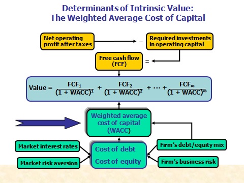
One option (if beta is given)

Another option (if dividend is given):
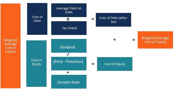
WACC Formula
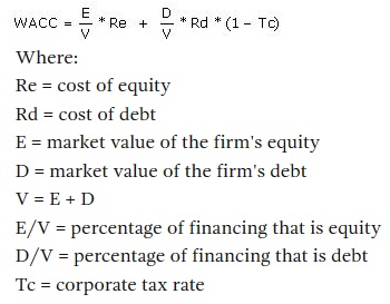
WACC calculator (with preferred stock, annual coupon bond)
(www.jufinance.com/wacc)
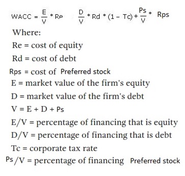
WACC calculator (with preferred stock, semi-annual coupon bond)
(www.jufinance.com/wacc_1)
Discount rate to
figure out the value of projects is called WACC (weighted average cost of
capital)
WACC = weight of debt
* cost of debt + weight of equity *( cost of equity)
Wd=
total debt / Total capital = total borrowed / total capital
We=
total equity/ Total capital
Cost of debt =
rate(nper, coupon, -(price – flotation costs), 1000)*(1-tax rate)
Cost of Equity =
D1/(Po – Flotation Cost) + g
D1: Next period dividend;
Po: Current stock price; g: dividend growth rate
Note:
flotation costs = flotation percentage * price
Or
if beta is given, use CAPM model (refer to chapter 6)
Cost
of equity = risk free rate + beta *(market return – risk free rate)
Cost
of equity = risk free rate + beta * market risk premium
In Class Exercise
1. Firm AAA sold a noncallable bond now has 20 years to
maturity. 9.25% annual coupon rate, paid semiannually, sells at a
price = $1,075, par = $1,000. Tax rate = 40%, 0% flotation fee, calculate
after tax cost of debt (5.08%)
Answer:
·
before
tax cost of debt = rate(20*2, 9.25%*1000/2, -(1075-0%*1075), 1000)*2
·
after
tax cost of debt = rate(20*2, 9.25%*1000/2, -(1075-0%*1075), 1000)*2*(1-40%)
= 5.08%
2.
Firm AAA’s equity condition
is as follows. D1 = $1.25; P0 = $27.50; g =
5.00%; and Flotation = 6.00% of price. Calculate cost of equity (9.84%)
Answer:
·
Cost
of equity = 1.25/(27.5-6%*27.5)+5% = 9.84%
3.
Firm
AAA raised 10m from the capital market. In it, 3m is from the debt market and
the rest from the equity market. Calculate WACC.
Answer:
WACC=
(3/10)*5.08% + (7/10)*9.84%
Template is available at https://www.jufinance.com/wacc_1/
Assignment (due with
final):
Case study 5 - Chapter 9 Case study
(due with final)
(help
video: https://www.jufinance.com/video/fin534_case_5_2021_spring.mp4)
- posted
Details about how to derive the model mathematically
(FYI)
The Gordon growth model is a simple discounted cash flow (DCF)
model which can be used to value a stock, mutual fund, or even the entire
stock market. The model is named after Myron Gordon who first published
the model in 1959.
The Gordon model assumes that a financial security
pays a periodic dividend (D) which grows at a constant rate
(g). These growing dividend payments are assumed to continue forever.
The future dividend payments are discounted at the required rate of return
(r) to find the price (P) for the stock or fund.
Under these simple assumptions, the price of the
security is given by this equation:
![]()
In this equation, I’ve used the “0” subscript
on the price (P) and the “1” subscript on the dividend (D) to indicate
that the price is calculated at time zero and the dividend is the expected
dividend at the end of period one. However, the equation is commonly
written with these subscripts omitted.
Obviously, the assumptions built into this
model are overly simplistic for many real-world valuation problems. Many
companies pay no dividends, and, for those that do,
we may expect changing payout ratios or growth rates as the
business matures.
Despite
these limitations, I believe spending some time experimenting with the
Gordon model can help develop intuition about the relationship between
valuation and return.
Deriving
the Gordon Growth Model Equation
The Gordon growth model calculates the present value of
the security by summing an infinite series of discounted dividend payments
which follows the pattern shown here:
![]()
Multiplying both sides of the previous equation by
(1+g)/(1+r) gives:
![]()
We can then subtract the second equation from the first
equation to get:
![]()
Rearranging and simplifying:
![]()
![]()
Finally, we can simplify further to get the Gordon growth model
equation
dividend growth model:
Refer
to http://www.calculatinginvestor.com/2011/05/18/gordon-growth-model/
·
Now let’s apply this Dividend growth model in problem
solving.
P/E Ratio Summary by
industry (FYI) --- Thanks to Dr Damodaran
Data Used: Multiple data services
Date of Analysis: Data used is as of January 2021
Download as an excel file instead: http://www.stern.nyu.edu/~adamodar/pc/datasets/pedata.xls
For global datasets: http://www.stern.nyu.edu/~adamodar/New_Home_Page/data.html
|
Industry Name |
Number of firms |
Current PE |
Expected growth
- next 5 years |
PEG Ratio |
|
Advertising |
61 |
20.95 |
83.44% |
0.19 |
|
Aerospace/Defense |
72 |
291.56 |
5.78% |
3.55 |
|
Air Transport |
17 |
8.14 |
-14.27% |
NA |
|
Apparel |
51 |
22.38 |
13.60% |
1.63 |
|
Auto &
Truck |
19 |
164.37 |
18.80% |
8.87 |
|
Auto Parts |
52 |
27.43 |
12.42% |
2.92 |
|
Bank (Money
Center) |
7 |
8.46 |
5.27% |
2.83 |
|
Banks
(Regional) |
598 |
13.5 |
5.74% |
2.32 |
|
Beverage
(Alcoholic) |
23 |
45.64 |
17.53% |
2.06 |
|
Beverage (Soft) |
41 |
201.34 |
10.24% |
2.93 |
|
Broadcasting |
29 |
15.1 |
12.93% |
0.96 |
|
Brokerage &
Investment Banking |
39 |
21.14 |
8.88% |
1.81 |
|
Building
Materials |
42 |
28.19 |
15.28% |
1.43 |
|
Business &
Consumer Services |
169 |
38.25 |
12.28% |
3.28 |
|
Cable TV |
13 |
68.46 |
29.41% |
1.04 |
|
Chemical
(Basic) |
48 |
13.8 |
9.70% |
1.79 |
|
Chemical
(Diversified) |
5 |
13.89 |
5.55% |
2.35 |
|
Chemical
(Specialty) |
97 |
36.06 |
9.18% |
3.4 |
|
Coal &
Related Energy |
29 |
2.85 |
-20.90% |
NA |
|
Computer
Services |
116 |
45.38 |
9.98% |
1.86 |
|
Computers/Peripherals |
52 |
40.61 |
12.30% |
2.97 |
|
Construction
Supplies |
46 |
84.99 |
11.21% |
2.27 |
|
Diversified |
29 |
26.18 |
9.58% |
1.86 |
|
Drugs
(Biotechnology) |
547 |
31 |
18.96% |
1.14 |
|
Drugs
(Pharmaceutical) |
287 |
122.82 |
11.28% |
2.09 |
|
Education |
38 |
26.92 |
14.76% |
1.75 |
|
Electrical
Equipment |
122 |
51.61 |
1.85% |
15.93 |
|
Electronics (Consumer &
Office) |
22 |
57.06 |
20.95% |
0.66 |
|
Electronics
(General) |
157 |
81.09 |
15.15% |
2.72 |
|
Engineering/Construction |
61 |
27.42 |
11.33% |
2.38 |
|
Entertainment |
118 |
908.12 |
17.03% |
3.18 |
|
Environmental
& Waste Services |
86 |
538.13 |
11.58% |
3.72 |
|
Farming/Agriculture |
32 |
26.45 |
17.84% |
1.38 |
|
Financial Svcs.
(Non-bank & Insurance) |
235 |
24.3 |
13.59% |
1.08 |
|
Food Processing |
101 |
268.11 |
13.87% |
1.54 |
|
Food Wholesalers |
18 |
320.61 |
11.97% |
0.71 |
|
Furn/Home
Furnishings |
40 |
29.97 |
15.23% |
1.25 |
|
Green &
Renewable Energy |
25 |
56 |
12.25% |
5.25 |
|
Healthcare
Products |
265 |
330.73 |
16.92% |
2.81 |
|
Healthcare Support
Services |
129 |
101.84 |
16.32% |
1.03 |
|
Heathcare
Information and Technology |
139 |
189.47 |
21.56% |
1.82 |
|
Homebuilding |
30 |
19.46 |
16.91% |
0.67 |
|
Hospitals/Healthcare
Facilities |
32 |
72.23 |
13.75% |
1.33 |
|
Hotel/Gaming |
66 |
51.99 |
-15.51% |
NA |
|
Household
Products |
140 |
592.23 |
9.46% |
2.98 |
|
Information
Services |
77 |
102.24 |
11.15% |
4.86 |
|
Insurance
(General) |
21 |
65.34 |
33.98% |
0.63 |
|
Insurance
(Life) |
26 |
18.97 |
7.81% |
1 |
|
Insurance
(Prop/Cas.) |
55 |
44.23 |
8.58% |
1.55 |
|
Investments
& Asset Management |
348 |
480.92 |
10.73% |
1.64 |
|
Machinery |
125 |
59.51 |
12.27% |
2.63 |
|
Metals &
Mining |
86 |
30.21 |
72.06% |
0.51 |
|
Office
Equipment & Services |
22 |
16.09 |
8.16% |
3.09 |
|
Oil/Gas
(Integrated) |
3 |
33.88 |
7.20% |
7.29 |
|
Oil/Gas
(Production and Exploration) |
278 |
25.15 |
-25.81% |
NA |
|
Oil/Gas
Distribution |
57 |
10.84 |
6.69% |
2.28 |
|
Oilfield Svcs/Equip. |
135 |
40.3 |
7.98% |
0.34 |
|
Packaging &
Container |
26 |
25.24 |
11.40% |
2.37 |
|
Paper/Forest
Products |
15 |
20.06 |
7.00% |
1.96 |
|
Power |
55 |
21.48 |
7.02% |
2.96 |
|
Precious Metals |
93 |
19.65 |
12.85% |
1.52 |
|
Publishing
& Newspapers |
29 |
48 |
9.21% |
4.51 |
|
R.E.I.T. |
238 |
49.79 |
2.10% |
17.69 |
|
Real Estate (Development) |
25 |
31.02 |
14.50% |
1.1 |
|
Real Estate
(General/Diversified) |
11 |
40.16 |
-3.24% |
NA |
|
Real Estate
(Operations & Services) |
61 |
1199.26 |
21.97% |
1.01 |
|
Recreation |
69 |
39.3 |
22.98% |
3.22 |
|
Reinsurance |
2 |
9.56 |
30.10% |
0.51 |
|
Restaurant/Dining |
79 |
70.43 |
12.54% |
3.93 |
|
Retail
(Automotive) |
30 |
30.46 |
13.29% |
1.27 |
|
Retail
(Building Supply) |
15 |
152.69 |
18.72% |
1.23 |
|
Retail
(Distributors) |
85 |
41.38 |
9.94% |
2.59 |
|
Retail
(General) |
17 |
23.23 |
2.14% |
10.77 |
|
Retail (Grocery and Food) |
14 |
40.6 |
12.26% |
0.78 |
|
Retail (Online) |
75 |
133.68 |
20.17% |
3.51 |
|
Retail (Special
Lines) |
85 |
30.51 |
9.91% |
4.19 |
|
Rubber&
Tires |
3 |
39.19 |
7.45% |
1.76 |
|
Semiconductor |
70 |
1291.42 |
13.63% |
2.3 |
|
Semiconductor
Equip |
40 |
108.68 |
24.68% |
1.14 |
|
Shipbuilding
& Marine |
11 |
23.47 |
11.30% |
2.19 |
|
Shoe |
11 |
31.53 |
15.84% |
4.45 |
|
Software
(Entertainment) |
101 |
100.59 |
19.72% |
1.67 |
|
Software
(Internet) |
36 |
92.26 |
23.68% |
1.36 |
|
Software
(System & Application) |
388 |
193.65 |
22.61% |
1.73 |
|
Steel |
32 |
76.29 |
1.93% |
8.99 |
|
Telecom
(Wireless) |
16 |
29.65 |
10.30% |
4.67 |
|
Telecom.
Equipment |
96 |
69.36 |
14.07% |
1.57 |
|
Telecom.
Services |
58 |
158.41 |
6.90% |
2.17 |
|
Tobacco |
15 |
28.53 |
9.83% |
2.48 |
|
Transportation |
21 |
27.84 |
11.20% |
2.77 |
|
Transportation
(Railroads) |
6 |
25.54 |
9.37% |
2.87 |
|
Trucking |
35 |
30.51 |
4.76% |
5.53 |
|
Utility
(General) |
16 |
20.24 |
4.95% |
3.21 |
|
Utility (Water) |
17 |
54.77 |
8.56% |
4.83 |
|
Total Market |
7582 |
109.79 |
11.64% |
2.35 |
|
Total Market
(without financials) |
6253 |
103.33 |
12.17% |
2.5 |
Walmart
Inc (NYSE:WMT) WACC %:3.36% As of Today (6/25/2021)
As of today,
Walmart Inc's weighted average cost of capital is 3.36%. Walmart Inc's ROIC % is 8.81% (calculated
using TTM income statement data). Walmart Inc generates higher returns on
investment than it costs the company to raise the capital needed for that
investment. It is earning excess returns. A firm that expects to continue
generating positive excess returns on new investments in the future will see
its value increase as growth increases.
https://www.gurufocus.com/term/wacc/WMT/WACC/Walmart%2BInc
Amazon.com
Inc (NAS:AMZN) WACC %:8.06% As of Today (6/25/2021)
As of today,
Amazon.com Inc's weighted average cost of capital is 8.06%.
Amazon.com Inc's ROIC % is 13.47% (calculated
using TTM income statement data). Amazon.com Inc generates higher returns on
investment than it costs the company to raise the capital needed for that
investment. It is earning excess returns. A firm that expects to continue
generating positive excess returns on new investments in the future will see
its value increase as growth increases.
https://www.gurufocus.com/term/wacc/AMZN/WACC-Percentage/Amazon.com%20Inc
|
Ticker |
Company |
Market Cap (M) |
WACC % |
|
AMZN |
Amazon.com Inc |
$1,555,758.24 |
8.07 |
|
HKSE:09988 |
Alibaba Group |
$631,785.07 |
6.45 |
|
HKSE:03690 |
Meituan |
$252,602.83 |
7.63 |
|
PDD |
Pinduoduo Inc |
$197,512.71 |
7.63 |
|
HKSE:09618 |
JD.com Inc |
$137,594.60 |
6.32 |
|
CPNG |
Coupang Inc |
$83,132.87 |
0 |
|
MELI |
MercadoLibre Inc |
$77,305.56 |
10.45 |
|
CVNA |
Carvana Co |
$49,385.49 |
17.6 |
|
EBAY |
eBay Inc |
$37,968.87 |
7.71 |
|
CHWY |
Chewy Inc |
$35,322.56 |
7.64 |
Tesla (NAS:TSLA) WACC
%:13.42% (6/25/2021)
As of today, Tesla’s weighted average cost of
capital is 13.42%. Apple Inc's ROIC % is 5.67% (calculated
using TTM income statement data).
https://www.gurufocus.com/term/wacc/TSLA/WACC/Tesla%2Binc
|
Competitive Comparison Data |
|||
|
Ticker |
Company |
Market Cap (M) |
WACC % |
|
TSLA |
Tesla Inc |
$665,879.17 |
14.35 |
|
TSE:7203 |
Toyota Motor Corp |
$208,955.81 |
2.33 |
|
XTER:VOW3 |
Volkswagen AG |
$128,507.15 |
2.73 |
|
XTER:DAI |
Daimler AG |
$90,436.93 |
2.62 |
|
GM |
General Motors Co |
$85,388.49 |
4.73 |
|
XTER:NSU |
Audi AG |
$84,294.28 |
5.62 |
|
LTS:0FG8 |
Audi AG |
$82,752.31 |
5.62 |
|
HKSE:01211 |
BYD Co Ltd |
$76,495.24 |
6.81 |
|
NIO |
NIO Inc |
$70,930.41 |
7.61 |
|
XTER:BMW |
Bayerische Motoren Werke AG |
$59,930.08 |
3.36 |
Apple
Inc (NAS:AAPL) WACC %:8.89% As of Today (6/25/2021)
As of today,
Apple Inc's weighted average cost of capital is 9.04%. Apple
Inc's ROIC % is 29.77% (calculated
using TTM income statement data). Apple Inc generates higher returns on
investment than it costs the company to raise the capital needed for that
investment. It is earning excess returns. A firm that expects to continue
generating positive excess returns on new investments in the future will see
its value increase as growth increases.
https://www.gurufocus.com/term/wacc/AAPL/WACC/Apple%2Binc
|
Industry
Name |
Number
of Firms |
Cost
of Equity |
E/(D+E) |
Cost
of Debt |
Tax
Rate |
D/(D+E) |
Cost
of Capital |
|
Advertising |
40 |
8.27% |
57.51% |
6.91% |
6.38% |
42.49% |
6.99% |
|
Aerospace/Defense |
87 |
7.91% |
84.42% |
3.91% |
11.59% |
15.58% |
7.14% |
|
Air Transport |
17 |
7.54% |
58.48% |
3.91% |
24.57% |
41.52% |
5.64% |
|
Apparel |
51 |
7.58% |
74.52% |
3.91% |
10.35% |
25.48% |
6.40% |
|
Auto & Truck |
18 |
8.49% |
40.31% |
3.61% |
8.15% |
59.69% |
5.06% |
|
Auto Parts |
62 |
7.68% |
77.94% |
3.91% |
7.71% |
22.06% |
6.64% |
|
Bank (Money Center) |
11 |
5.65% |
38.87% |
3.61% |
27.31% |
61.13% |
3.87% |
|
Banks (Regional) |
612 |
4.96% |
63.02% |
3.61% |
25.57% |
36.98% |
4.14% |
|
Beverage (Alcoholic) |
28 |
9.15% |
79.27% |
3.91% |
10.12% |
20.73% |
7.87% |
|
Beverage (Soft) |
35 |
5.99% |
81.26% |
3.91% |
6.41% |
18.74% |
5.42% |
|
Broadcasting |
27 |
8.10% |
47.13% |
3.91% |
17.18% |
52.87% |
5.39% |
|
Brokerage & Investment
Banking |
42 |
8.70% |
31.26% |
3.91% |
14.56% |
68.74% |
4.76% |
|
Building Materials |
39 |
8.04% |
82.33% |
3.91% |
23.34% |
17.67% |
7.15% |
|
Business & Consumer Services |
169 |
8.35% |
78.47% |
3.91% |
11.09% |
21.53% |
7.19% |
|
Cable TV |
14 |
7.09% |
65.34% |
3.61% |
22.23% |
34.66% |
5.58% |
|
Chemical (Basic) |
38 |
8.49% |
70.78% |
3.91% |
9.76% |
29.22% |
6.88% |
|
Chemical
(Diversified) |
7 |
12.74% |
78.63% |
4.66% |
11.66% |
21.37% |
10.78% |
|
Chemical (Specialty) |
99 |
8.07% |
77.52% |
3.91% |
9.64% |
22.48% |
6.93% |
|
Coal & Related Energy |
30 |
8.75% |
68.77% |
8.16% |
4.94% |
31.23% |
7.96% |
|
Computer Services |
111 |
8.00% |
76.43% |
3.91% |
9.40% |
23.57% |
6.82% |
|
Computers/Peripherals |
58 |
7.54% |
84.62% |
3.91% |
5.03% |
15.38% |
6.84% |
|
Construction Supplies |
49 |
8.10% |
75.49% |
3.91% |
17.36% |
24.51% |
6.85% |
|
Diversified |
24 |
8.48% |
75.48% |
3.61% |
12.09% |
24.52% |
7.07% |
|
Drugs (Biotechnology) |
459 |
9.72% |
86.33% |
8.16% |
1.36% |
13.67% |
9.24% |
|
Drugs (Pharmaceutical) |
185 |
8.55% |
87.24% |
6.91% |
2.11% |
12.76% |
8.13% |
|
Education |
34 |
8.27% |
72.03% |
3.91% |
8.24% |
27.97% |
6.79% |
|
Electrical Equipment |
118 |
7.92% |
86.32% |
4.66% |
5.06% |
13.68% |
7.32% |
|
Electronics (Consumer & Office) |
24 |
7.96% |
93.51% |
4.66% |
5.98% |
6.49% |
7.67% |
|
Electronics (General) |
167 |
7.17% |
86.98% |
3.91% |
8.34% |
13.02% |
6.63% |
|
Engineering/Construction |
49 |
8.86% |
77.09% |
3.91% |
13.37% |
22.91% |
7.51% |
|
Entertainment |
90 |
8.26% |
74.77% |
3.91% |
5.45% |
25.23% |
6.93% |
|
Environmental & Waste
Services |
87 |
6.87% |
74.15% |
4.66% |
4.45% |
25.85% |
6.01% |
|
Farming/Agriculture |
34 |
6.19% |
64.29% |
3.91% |
7.69% |
35.71% |
5.04% |
|
Financial Svcs.
(Non-bank & Insurance) |
264 |
5.49% |
8.83% |
3.61% |
19.89% |
91.17% |
2.99% |
|
Food Processing |
87 |
5.84% |
76.44% |
3.91% |
15.13% |
23.56% |
5.17% |
|
Food Wholesalers |
15 |
11.48% |
72.75% |
3.91% |
11.91% |
27.25% |
9.16% |
|
Furn/Home Furnishings |
31 |
6.42% |
78.21% |
3.91% |
12.56% |
21.79% |
5.67% |
|
Green & Renewable Energy |
22 |
8.51% |
50.45% |
3.91% |
2.41% |
49.55% |
5.77% |
|
Healthcare Products |
251 |
7.19% |
85.41% |
4.66% |
4.79% |
14.59% |
6.66% |
|
Healthcare Support Services |
115 |
6.97% |
80.11% |
3.91% |
13.69% |
19.89% |
6.17% |
|
Heathcare Information and
Technology |
112 |
7.38% |
83.83% |
3.91% |
5.96% |
16.17% |
6.67% |
|
Homebuilding |
32 |
8.04% |
71.61% |
3.91% |
23.86% |
28.39% |
6.60% |
|
Hospitals/Healthcare Facilities |
35 |
8.40% |
36.16% |
3.91% |
10.57% |
63.84% |
4.93% |
|
Hotel/Gaming |
70 |
7.18% |
71.48% |
3.91% |
14.01% |
28.52% |
5.98% |
|
Household Products |
131 |
7.47% |
82.63% |
3.91% |
7.35% |
17.37% |
6.69% |
|
Information Services |
61 |
6.89% |
86.42% |
3.91% |
15.90% |
13.58% |
6.36% |
|
Insurance (General) |
21 |
6.39% |
72.20% |
3.61% |
14.71% |
27.80% |
5.38% |
|
Insurance (Life) |
25 |
7.53% |
63.67% |
3.61% |
15.32% |
36.33% |
5.79% |
|
Insurance (Prop/Cas.) |
50 |
6.67% |
79.10% |
3.61% |
18.50% |
20.90% |
5.85% |
|
Investments & Asset
Management |
165 |
7.43% |
70.38% |
3.91% |
8.30% |
29.62% |
6.11% |
|
Machinery |
126 |
8.25% |
83.51% |
3.91% |
14.05% |
16.49% |
7.38% |
|
Metals & Mining |
102 |
8.01% |
76.61% |
6.91% |
1.66% |
23.39% |
7.37% |
|
Office Equipment & Services |
24 |
9.39% |
65.94% |
3.91% |
18.37% |
34.06% |
7.20% |
|
Oil/Gas (Integrated) |
5 |
9.38% |
86.74% |
3.11% |
10.96% |
13.26% |
8.45% |
|
Oil/Gas (Production and
Exploration) |
311 |
8.80% |
70.47% |
6.91% |
2.18% |
29.53% |
7.76% |
|
Oil/Gas Distribution |
16 |
8.54% |
51.70% |
3.91% |
4.84% |
48.30% |
5.85% |
|
Oilfield Svcs/Equip. |
130 |
8.64% |
76.35% |
4.66% |
5.27% |
23.65% |
7.44% |
|
Packaging & Container |
25 |
6.16% |
66.57% |
3.61% |
22.37% |
33.43% |
5.02% |
|
Paper/Forest Products |
21 |
8.50% |
71.42% |
3.91% |
14.18% |
28.58% |
6.92% |
|
Power |
61 |
4.97% |
56.70% |
3.61% |
20.31% |
43.30% |
4.01% |
|
Precious Metals |
111 |
7.30% |
84.85% |
8.16% |
2.16% |
15.15% |
7.14% |
|
Publishing & Newspapers |
41 |
7.59% |
69.21% |
3.91% |
11.92% |
30.79% |
6.17% |
|
R.E.I.T. |
244 |
5.76% |
56.02% |
3.61% |
1.96% |
43.98% |
4.43% |
|
Real Estate (Development) |
20 |
6.22% |
68.82% |
3.91% |
5.80% |
31.18% |
5.21% |
|
Real Estate
(General/Diversified) |
10 |
6.20% |
80.90% |
3.91% |
12.77% |
19.10% |
5.58% |
|
Real Estate (Operations &
Services) |
60 |
7.60% |
68.16% |
3.91% |
8.82% |
31.84% |
6.13% |
|
Recreation |
70 |
6.73% |
77.17% |
3.91% |
10.16% |
22.83% |
5.87% |
|
Reinsurance |
3 |
5.06% |
78.29% |
3.11% |
10.92% |
21.71% |
4.47% |
|
Restaurant/Dining |
81 |
6.73% |
75.64% |
3.91% |
14.99% |
24.36% |
5.81% |
|
Retail (Automotive) |
25 |
7.55% |
56.83% |
3.91% |
19.04% |
43.17% |
5.57% |
|
Retail (Building Supply) |
8 |
6.76% |
84.85% |
3.91% |
15.36% |
15.15% |
6.19% |
|
Retail (Distributors) |
92 |
8.25% |
68.69% |
3.91% |
14.20% |
31.31% |
6.59% |
|
Retail (General) |
18 |
7.74% |
76.25% |
3.91% |
22.96% |
23.75% |
6.61% |
|
Retail (Grocery and Food) |
14 |
6.00% |
54.44% |
3.91% |
21.04% |
45.56% |
4.62% |
|
Retail (Online) |
61 |
8.41% |
89.76% |
3.91% |
7.57% |
10.24% |
7.86% |
|
Retail (Special Lines) |
106 |
8.05% |
65.36% |
3.91% |
22.01% |
34.64% |
6.29% |
|
Rubber& Tires |
4 |
7.25% |
56.18% |
3.91% |
7.91% |
43.82% |
5.38% |
|
Semiconductor |
72 |
8.37% |
88.42% |
3.91% |
8.04% |
11.58% |
7.74% |
|
Semiconductor Equip |
45 |
7.40% |
89.66% |
3.91% |
8.51% |
10.34% |
6.94% |
|
Shipbuilding & Marine |
9 |
9.22% |
68.05% |
8.16% |
8.31% |
31.95% |
8.26% |
|
Shoe |
11 |
6.89% |
91.20% |
3.91% |
16.75% |
8.80% |
6.54% |
|
Software (Entertainment) |
13 |
6.94% |
93.94% |
3.91% |
2.21% |
6.06% |
6.70% |
|
Software (Internet) |
305 |
8.52% |
96.79% |
4.66% |
2.50% |
3.21% |
8.36% |
|
Software (System &
Application) |
255 |
7.93% |
87.61% |
3.91% |
3.98% |
12.39% |
7.32% |
|
Steel |
37 |
11.64% |
73.41% |
4.66% |
7.05% |
26.59% |
9.49% |
|
Telecom (Wireless) |
18 |
9.02% |
45.46% |
3.91% |
7.95% |
54.54% |
5.72% |
|
Telecom. Equipment |
104 |
7.67% |
82.83% |
3.91% |
8.12% |
17.17% |
6.86% |
|
Telecom. Services |
66 |
7.91% |
55.70% |
3.91% |
8.05% |
44.30% |
5.72% |
|
Tobacco |
24 |
8.82% |
85.37% |
3.91% |
5.25% |
14.63% |
7.97% |
|
Transportation |
18 |
7.23% |
76.91% |
3.91% |
21.92% |
23.09% |
6.25% |
|
Transportation (Railroads) |
8 |
7.52% |
81.52% |
3.61% |
23.82% |
18.48% |
6.64% |
|
Trucking |
30 |
8.50% |
58.89% |
3.91% |
20.56% |
41.11% |
6.23% |
|
Utility
(General) |
18 |
3.90% |
59.79% |
3.11% |
30.89% |
40.21% |
3.28% |
|
Utility (Water) |
23 |
4.15% |
72.39% |
3.61% |
15.09% |
27.61% |
3.76% |
|
Total Market |
7247 |
7.49% |
62.89% |
3.91% |
10.04% |
37.11% |
5.81% |
|
Total Market (no financials) |
6057 |
7.84% |
76.49% |
3.91% |
7.92% |
23.51% |
6.69% |
http://people.stern.nyu.edu/adamodar/New_Home_Page/datafile/wacc.htm
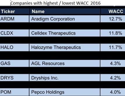
·
.
Discounted Cash Flow (DCF, FYI)
By JASON FERNANDO Reviewed by KHADIJA KHARTIT Updated Mar 13, 2021
https://www.investopedia.com/terms/d/dcf.asp
(video)
What
Is Discounted Cash Flow (DCF)?
Discounted cash flow (DCF) is a
valuation method used to estimate the value of an investment based on its
expected future cash flows. DCF analysis attempts to figure out the value of
an investment today, based on projections of how much money it will generate
in the future.
This applies to investment
decisions of investors in companies or securities, such as acquiring a
company, investing in a technology startup, or buying a stock, and for
business owners and managers looking to make capital budgeting or operating
expenditures decisions such as opening a new factory, purchasing or leasing
new equipment.
KEY
TAKEAWAYS
· Discounted cash flow (DCF) helps determine the value of an investment based on its future cash flows.
· The present value of expected future cash flows is arrived at by using a discount rate to calculate the discounted cash flow (DCF).
· If the discounted cash flow (DCF) is above the current cost of the investment, the opportunity could result in positive returns.
· Companies typically use the weighted average cost of capital for the discount rate, as it takes into consideration the rate of return expected by shareholders.
· The DCF has limitations, primarily that it relies on estimations on future cash flows, which could prove to be inaccurate.
How
Discounted Cash Flow Works
The purpose of DCF analysis is
to estimate the money an investor would receive from an investment, adjusted
for the time value of money. The time value of money assumes that a dollar
today is worth more than a dollar tomorrow because it can be invested. As
such, a DCF analysis is appropriate in any situation where a person is paying
money in the present with expectations of receiving more money in the future.
For example, assuming a 5%
annual interest rate, $1.00 in a savings account will be worth $1.05 in a
year. Similarly, if a $1 payment is delayed for a year, its present value is $.95
because it cannot be put in your savings account to earn interest.
DCF analysis finds the present
value of expected future cash flows using a discount rate. Investors can use
the concept of the present value of money to determine whether future cash flows
of an investment or project are equal to or greater than the value of the
initial investment. If the value calculated through DCF is higher than the
current cost of the investment, the opportunity should be considered.
In order to conduct a DCF analysis,
an investor must make estimates about future cash flows and the ending value
of the investment, equipment, or other asset. The investor must also
determine an appropriate discount rate for the DCF model, which will vary
depending on the project or investment under consideration, such as the
company or investor's risk profile and the conditions of the capital markets.
If the investor cannot access the future cash flows, or the project is very
complex, DCF will not have much value and alternative models should be
employed.
Discounted Cash Flow Formula
The formula for DCF is:
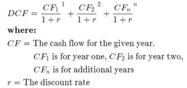
Example
of Discounted Cash Flow
When a company looks to analyze
whether it should invest in a certain project or purchase new equipment, it
usually uses its weighted average cost of capital (WACC) as the discount rate
when evaluating the DCF. The WACC incorporates the average rate of return
that shareholders in the firm are expecting for the given year.
You are looking to invest in a
project, and your company's WACC is 5%, so you will use 5% as your discount
rate. The initial investment is $11 million and the project will last for
five years, with the following estimated cash flows per year:
Cash Flow
Year Cash Flow
1 $1 million
2 $1 million
3 $4 million
4 $4 million
5 $6 million
Therefore, the discounted cash
flows for the project are:
Discounted Cash Flow
Year Cash Flow Discounted
Cash Flow (nearest $)
1 $1 million $952,381
2 $1 million $907,029
3 $4 million $3,455,350
4 $4 million $3,290,810
5 $6 million $4,701,157
If we sum up all of the
discounted cash flows, we get a value of $13,306,728. Subtracting the initial
investment of $11 million, we get a net present value (NPV) of $2,306,728.
Because this is a positive number, the cost of the investment today is worth
it as the project will generate positive discounted cash flows above the
initial cost. If the project had cost $14 million, the NPV would have been
-$693,272, indicating that the cost of the investment would not be worth it.
Dividend discount models, such as the Gordon
Growth Model (GGM), for valuing stocks are examples of using discounted cash
flows.
Disadvantages
of Discounted Cash Flow
The main limitation of DCF is
that it requires making many assumptions. For one, an investor would have to
correctly estimate the future cash flows from an investment or project. The
future cash flows would rely on a variety of factors, such as market demand,
the status of the economy, technology, competition, and unforeseen threats or
opportunities.
Estimating future cash flows
too high could result in choosing an investment that might not pay off in the
future, hurting profits. Estimating cash flows too low, making an investment
appear costly, could result in missed opportunities. Choosing a discount rate
for the model is also an assumption and would have to be estimated correctly
for the model to be worthwhile.
How
do you calculate discounted cash flow (DCF)?
Calculating the DCF of an
investment involves three basic steps. First, you forecast the expected cash
flows from the investment. Second, you select a discount rate, typically
based on the cost of financing the investment or the opportunity cost
presented by alternative investments. The third and final step is to discount
the forecasted cash flows back to the present day, using a financial
calculator, a spreadsheet, or a manual calculation.
What
is an example of a DCF calculation?
To illustrate, suppose you have
a discount rate of 10% and an investment opportunity that would produce $100
per year for the following three years. Your goal is to calculate the value
today—in other words, the “present value”—of this stream of cashflows. Since
money in the future is worth less than money today, you reduce the present
value of each of these cash flows by your 10% discount rate.
Specifically, the first year’s
cash flow is worth $90.91 today, the second year’s cash flow is worth $82.64
today, and the third year’s cash flow is worth $75.13 today. Adding up these
three cashflows, you conclude that the DCF of the investment is $248.68.
Chapter 10 The
Basics of Capital Budgeting
Topics in Chapter 10:
· Overview
and “vocabulary”
· Capital
Budgeting Methods
o
NPV
o
IRR
o
Payback
o
MIRR
o
Profitable index
o
Discounted payback
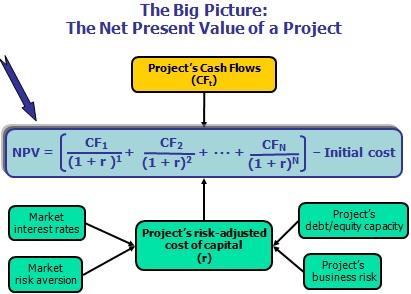
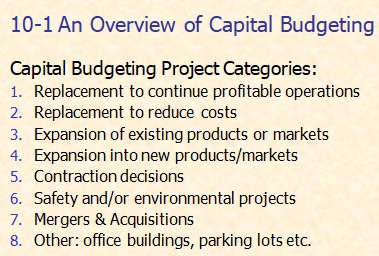
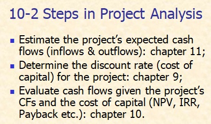
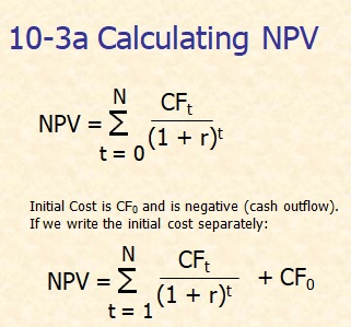
Math equation:
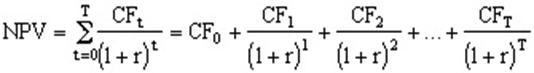
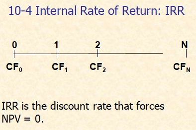
Math equation:
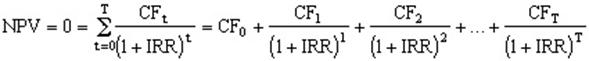
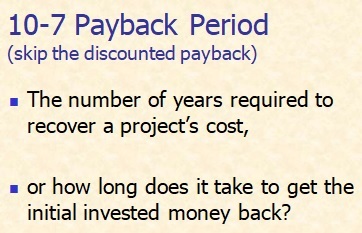
Math equation:
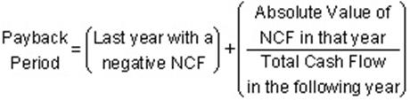
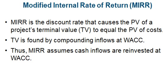
Math equation:
MIRR = (FVCI/PVCO)1/n-1
·
Where MIRR is the modified internal rate of
return, FVCI is the sum of future values of all net cash flows at
the end of the project, PVCO is the initial investment, and n is
the number of periods
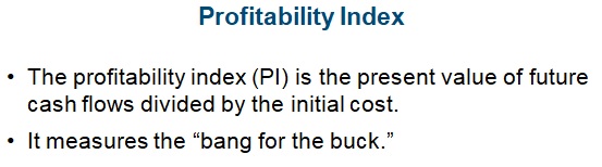
Math equation:
Profitability Index = Present
Value of Future Cash Flows ÷ Initial Investment in the Project.
Excel Syntax:
1. NPV Excel syntax
Syntax
NPV(rate,value1,value2, ...)
Rate is the rate of discount over the
length of one period.
Value1, value2,
... are 1 to
29 arguments representing the payments and income.
· Value1, value2, ... must be equally spaced in time
and occur at the end of each period. NPV uses the
order of value1, value2, ... to interpret the order of cash flows.
Be sure to enter your payment and income values in the correct sequence.
2. IRR Excel syntax
Syntax
IRR(values, guess)
Values is an array or a reference to cells that
contain numbers for which you want to calculate the internal rate of return.
Guess is a number that you guess is close
to the result of IRR.
3) MIRR Excel syntax
Syntax
MIRR (values, finance_rate,
reinvest_rate)
·
values - Array or reference to cells that contain cash flows.
·
finance_rate - Required rate of return (discount rate) as
percentage.
·
reinvest_rate - Interest rate received on cash flows reinvested
as percentage.
NPV,
IRR, Payback Period, MIRR, Discounted payback calculator www.jufinance.com/capital
Template
in Excel https://www.jufinance.com/npv_1/
In class exercise: (none)
Let’s use the case study as in class exercise
Assignment (due with
final):
(help video: https://www.jufinance.com/video/fin534_case_6_2021_spring.mp4) - Posted
Simple
Rules’ for Running a Business
From the 20-page cellphone contract to the five-pound employee
handbook, even the simple things seem to be getting more complicated.
Companies have been
complicating things for themselves, too—analyzing
hundreds of factors when making decisions, or consulting reams of data to
resolve every budget dilemma. But those requirements might be wasting time
and muddling priorities.
So argues Donald Sull, a lecturer at the Sloan School of Management at the
Massachusetts Institute of Technology who has also worked for McKinsey &
Co. and Clayton, Dubilier &
Rice LLC. In the book Simple Rules: How to Thrive in a Complex World,
out this week from Houghton Mifflin Harcourt HMHC -1.36%, he and Kathleen Eisenhardt of Stanford University claim that
straightforward guidelines lead to better results than complex formulas.
Mr. Sull recently spoke with At Work about
what companies can do to simplify, and why five basic rules can beat a
50-item checklist. Edited excerpts:
WSJ: Where, in the business context, might “simple
rules” help
more than a complicated approach?
Donald Sull: Well, a common decision that people face in organizations is
capital allocation. In many organizations, there will be thick procedure
books or algorithms–one company I worked with had an
algorithm that had almost 100 variables for every project. These are very
cumbersome approaches to making decisions and can waste time. Basically, any
decision about how to focus resources—either people
or money or attention—can benefit from simple rules.
WSJ: Can you give an example of how that simplification works in a
company?
Sull: There’s a
German company called Weima GmBH that
makes shredders. At one point, they were getting about 10,000 requests and
could only fill about a thousand because of technical capabilities, so they
had this massive problem of sorting out which of these proposals to pursue.
They had a very detailed checklist with 40 or 50 items. People
had to gather data and if there were gray areas the proposal would go to
management. But because the data was hard to obtain and there were so many
different pieces, people didn’t always fill out the
checklists completely. Then management had to discuss a lot of these
proposals personally because there was incomplete data. So top management is
spending a disproportionate amount of time discussing this low-level stuff.
Then Weima came up with guidelines that the
frontline sales force and engineers could use to quickly decide whether a
request fell in the “yes,” “no” or “maybe” category. They did it with five
rules only, stuff like “Weima had to collect at least 70% of the
price before the unit leaves the factory.”
After that, only the “maybes” were sent to management. This
dramatically decreased the amount of time management spend evaluating these
projects–that time was decreased by almost a factor
of 10.
Or, take Frontier Dental Laboratories in Canada. They were
working with a sales force of two covering the entire North American market.
Limiting their sales guidelines to a few factors that made someone likely to
be receptive to Frontier—stuff like “dentists
who have their own practice” and “dentists
with a website”—helped focus their efforts and
increase sales 42% in a declining market.
WSJ: Weima used
five factors—is that the optimal number? And how do
you choose which rules to follow?
Sull: You should
have four to six rules. Any more than that, you’ll spend too much time trying to follow
everything perfectly. The entire reason simple rules help is because they
force you to prioritize the goals that matter. They’re easy to remember, they
don’t confuse or stress you, they save time.
They should be tailored to your specific goals, so you choose
the rules based on what exactly you’re trying to
achieve. And you should of course talk to others. Get information from
different sources, and ask them for the top things that worked for them. But
focus on whether what will work for you and your circumstances.
WSJ: Is there a business leader you can point to who has embraced
the “simple rules” guideline?
Donald Sull: Let’s look at when Alex Behring took over America Latina Logistica SARUMO3.BR +1.59%, the Brazilian
railway and logistics company. With a budget of $15 million, how do you
choose among $200 million of investment requests, all of which are valid?
The textbook business-school answer to this is that you run the
NPV (net present value) test on each project and rank-order them by NPV. Alex
Behring knows this. He was at the top of the class at Harvard Business School.
But instead, he decided what the most important
goals were. You can’t achieve everything at once. In their case, their
priorities were removing bottlenecks on growing revenues and minimizing
upfront expenditure. So when allocating money, they had a bias for projects
that both addressed the bottleneck problem and, for example, used existing
tracks and trains.
Similarly, the global-health arm of the Gates Foundation gets
many, many funding requests. But since they know that their goal is to have
the most impact worldwide, they focus on projects in developing countries
because that’s where the money will stretch farther.
Chapter 11 Cash
Flow Estimation and Risk Analysis
Topics in Chapter 11:
· Estimating
cash flows
o
Relevant cash flows
o
Working capital treatment
o
Tax Depreciation
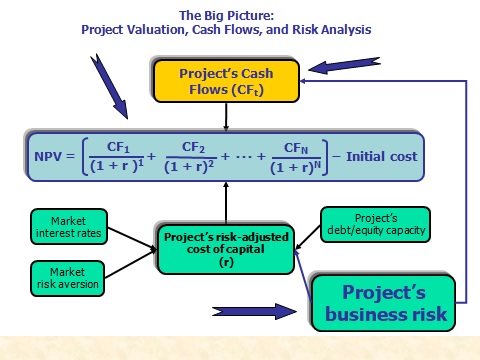
This is the Discounted
Cash Flow approach.
What is Discounted Cash
Flow (DCF)? (video)
11-2: an expansion
project
Detail:
Project L is the application of a radically new liquid
nano-coating technology to a new type of solar water heater module, which will
be manufactured under a 4-year license from a university. In this section, we
show how these cash flows are estimated (we only show this for Project L
here). It’s not clear how well the water heater will work, how strong demand
for it will be, how long it will be before the product becomes obsolete, or
whether the license can be renewed after the initial 4 years. Still, the
water heater has the potential for being profitable, though it could also
fail miserably. GPC is a relatively large company and this is one of many
projects, so a failure would not bankrupt the firm but would hurt profits and
the stock’s price.
Information given as blow:
·
Units sold at year 1: 10,000; increase by 15%
after year 1;
·
Unit sales price at year 1: $1.50; increase by
4% after year 1;
·
Variable cost per unit at year 1: $1.07;
increase by 3% after year 1;
·
Fixed cost at year 1: $2,120; increase by 3%
after year 1;
·
Net working capital requirement
·
NWCt = 15%(Salest+1)
·
Tax rate = 40%.
·
Project cost of capital (WACC) = 10%.
|
Analysis of an Expansion
Project: Project L, Guyton Products Company (GPC) |
||||
|
Assumptions /
Inputs: Base Case |
||||
|
Equipment Cost |
$7,750 |
|||
|
Salvage Value of
Equipment at Year 4 |
$639 |
|||
|
Opportunity Cost |
0 |
|||
|
Externalities (Cannibalization) |
0 |
|||
|
Units Sold, Year 1 |
10,000 |
|||
|
Annual Change Units
sold after Year 1 |
15% |
|||
|
Sales Price Per
Unit, Year 1 |
$1.50 |
|||
|
Annual Change Sales
Price after Year 1 |
4% |
|||
|
Variable Cost per
Unit (VC), Year 1 |
$1.07 |
|||
|
Annual Change in VC
after Year 1 |
3% |
|||
|
Nonvariable Cost
(FC), Year 1 |
$2,120 |
|||
|
Annual Change in FC
after Year 1 |
3% |
|||
|
Project WACC |
10% |
|||
|
Tax Rate |
40% |
|||
|
Working Capital as %
of Next Year's Sales |
15% |
|||
Questions for discussion:
How to calculate OCF (operating cash flow)?
OCF
= (Sales Revenue –
COGS – SG&A – Depreciation)*(1-T) + Depreciation
= EBIT *(1-T) + Depreciation
= Net Operating Profit after Taxes +
Depreciation
What is incremental cash flow?
What is sunk cost? Example? Included in the cash flow?
What is opportunity cost? Example? Included in the cash flow?
Assignment
(due with final):
Incremental
Cash Flow
By
ALICIA TUOVILA Reviewed by THOMAS
BROCK Updated Sep 20, 2020
https://www.investopedia.com/terms/i/incrementalcashflow.asp (video)
What is Incremental Cash Flow?
Incremental
cash flow is the additional operating cash flow that an organization receives
from taking on a new project. A positive incremental cash flow means that the
company's cash flow will increase with the acceptance of the project. A
positive incremental cash flow is a good indication that an organization
should invest in a project.
KEY TAKEAWAYS
Incremental cash flow is the potential
increase or decrease in a company's cash flow related to the acceptance of a
new project or investment in a new asset.
Positive
incremental cash flow is a good sign that the investment is more profitable
to the company than the expenses it will incur.
Incremental
cash flow can be a good tool to assess whether to invest in a new project or
asset, but it should not be the only resource for assessing the new venture.
Understanding Incremental Cash Flow
There
are several components that must be identified when looking at incremental
cash flows: the initial outlay, cash flows from taking on the project,
terminal cost or value, and the scale and timing of the project. Incremental cash flow is the net cash
flow from all cash inflows and outflows over a specific time and between two
or more business choices.
For
example, a business may project the net effects on the cash flow statement of
investing in a new business line or expanding an existing business line. The
project with the highest incremental cash flow may be chosen as the better
investment option. Incremental cash
flow projections are required for calculating a project's net present value
(NPV), internal rate of return (IRR), and payback period. Projecting
incremental cash flows may also be helpful in the decision of whether to
invest in certain assets that will appear on the balance sheet.
Example of Incremental Cash Flow
As a
simple example, assume that a business is looking to develop a new product
line and has two alternatives, Line A and Line B. Over the next year, Line A
is projected to have revenues of $200,000 and expenses of $50,000. Line B is
expected to have revenues of $325,000 and expenses of $190,000. Line A would
require an initial cash outlay of $35,000, and Line B would require an
initial cash outlay of $25,000.
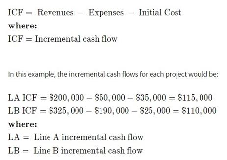
Even
though Line B generates more revenue than Line A, its resulting incremental
cash flow is $5,000 less than Line A's due to its larger expenses and initial
investment. If only using incremental cash flows as the determinant for
choosing a project, Line A is the better option.
Limitations of Incremental Cash Flow
The
simple example above explains the idea, but in practice, incremental cash
flows are extremely difficult to project. Besides the potential variables
within a business that could affect incremental cash flows, many external
variables are difficult or impossible to project. Market conditions,
regulatory policies, and legal policies may impact incremental cash flow in
unpredictable and unexpected ways. Another challenge is distinguishing
between cash flows from the project and cash flows from other business
operations. Without proper distinction, project selection can be made based
on inaccurate or flawed data.
Discounted Cash Flow (DCF)
By JASON FERNANDO Reviewed by KHADIJA KHARTIT Updated Mar 13, 2021
https://www.investopedia.com/terms/d/dcf.asp
(video)
What
Is Discounted Cash Flow (DCF)?
Discounted cash flow (DCF) is a
valuation method used to estimate the value of an investment based on its
expected future cash flows. DCF analysis attempts to figure out the value of
an investment today, based on projections of how much money it will generate
in the future.
This applies to investment
decisions of investors in companies or securities, such as acquiring a
company, investing in a technology startup, or buying a stock, and for
business owners and managers looking to make capital budgeting or operating
expenditures decisions such as opening a new factory, purchasing or leasing
new equipment.
KEY
TAKEAWAYS
· Discounted cash flow (DCF) helps determine the value of an investment based on its future cash flows.
· The present value of expected future cash flows is arrived at by using a discount rate to calculate the discounted cash flow (DCF).
· If the discounted cash flow (DCF) is above the current cost of the investment, the opportunity could result in positive returns.
· Companies typically use the weighted average cost of capital for the discount rate, as it takes into consideration the rate of return expected by shareholders.
· The DCF has limitations, primarily that it relies on estimations on future cash flows, which could prove to be inaccurate.
How
Discounted Cash Flow Works
The purpose of DCF analysis is
to estimate the money an investor would receive from an investment, adjusted
for the time value of money. The time value of money assumes that a dollar
today is worth more than a dollar tomorrow because it can be invested. As
such, a DCF analysis is appropriate in any situation where a person is paying
money in the present with expectations of receiving more money in the future.
For example, assuming a 5%
annual interest rate, $1.00 in a savings account will be worth $1.05 in a
year. Similarly, if a $1 payment is delayed for a year, its present value is
$.95 because it cannot be put in your savings account to earn interest.
DCF analysis finds the present
value of expected future cash flows using a discount rate. Investors can use
the concept of the present value of money to determine whether future cash
flows of an investment or project are equal to or greater than the value of
the initial investment. If the value calculated through DCF is higher than
the current cost of the investment, the opportunity should be considered.
In order to conduct a DCF
analysis, an investor must make estimates about future cash flows and the
ending value of the investment, equipment, or other asset. The investor must also
determine an appropriate discount rate for the DCF model, which will vary
depending on the project or investment under consideration, such as the
company or investor's risk profile and the conditions of the capital markets.
If the investor cannot access the future cash flows, or the project is very
complex, DCF will not have much value and alternative models should be
employed.
Discounted Cash Flow Formula
The formula for DCF is:
Example
of Discounted Cash Flow
When a company looks to analyze
whether it should invest in a certain project or purchase new equipment, it
usually uses its weighted average cost of capital (WACC) as the discount rate
when evaluating the DCF. The WACC incorporates the average rate of return
that shareholders in the firm are expecting for the given year.
You are looking to invest in a
project, and your company's WACC is 5%, so you will use 5% as your discount
rate. The initial investment is $11 million and the project will last for
five years, with the following estimated cash flows per year:
Cash Flow
Year Cash Flow
1 $1 million
2 $1 million
3 $4 million
4 $4 million
5 $6 million
Therefore, the discounted cash
flows for the project are:
Discounted Cash Flow
Year Cash Flow Discounted
Cash Flow (nearest $)
1 $1 million $952,381
2 $1 million $907,029
3 $4 million $3,455,350
4 $4 million $3,290,810
5 $6 million $4,701,157
If we sum up all of the
discounted cash flows, we get a value of $13,306,728. Subtracting the initial
investment of $11 million, we get a net present value (NPV) of $2,306,728.
Because this is a positive number, the cost of the investment today is worth
it as the project will generate positive discounted cash flows above the
initial cost. If the project had cost $14 million, the NPV would have been
-$693,272, indicating that the cost of the investment would not be worth it.
Dividend discount models, such as the Gordon
Growth Model (GGM), for valuing stocks are examples of using discounted cash
flows.
Disadvantages
of Discounted Cash Flow
The main limitation of DCF is
that it requires making many assumptions. For one, an investor would have to
correctly estimate the future cash flows from an investment or project. The
future cash flows would rely on a variety of factors, such as market demand,
the status of the economy, technology, competition, and unforeseen threats or
opportunities.
Estimating future cash flows
too high could result in choosing an investment that might not pay off in the
future, hurting profits. Estimating cash flows too low, making an investment
appear costly, could result in missed opportunities.
Choosing a discount rate for the model is also an assumption and would have
to be estimated correctly for the model to be worthwhile.
How
do you calculate discounted cash flow (DCF)?
Calculating the DCF of an
investment involves three basic steps. First, you forecast the expected cash
flows from the investment. Second, you select a discount rate, typically
based on the cost of financing the investment or the opportunity cost
presented by alternative investments. The third and final step is to discount
the forecasted cash flows back to the present day, using a financial
calculator, a spreadsheet, or a manual calculation.
What
is an example of a DCF calculation?
To illustrate, suppose you have
a discount rate of 10% and an investment opportunity that would produce $100
per year for the following three years. Your goal is to calculate the value
today—in other words, the “present value”—of this stream of cashflows. Since money in the future is worth less than
money today, you reduce the present value of each of these cash flows by your
10% discount rate.
Specifically, the first year’s
cash flow is worth $90.91 today, the second year’s cash flow is worth $82.64
today, and the third year’s cash flow is worth $75.13 today. Adding up these
three cashflows, you conclude that the DCF of the
investment is $248.68.
Chapter 14 Distribution to
Shareholders (deleted)
Topics in Chapter 14:
·
Theories of investor preferences
·
Clientele effect
·
Signaling effect
·
Residual distribution model
·
Stock repurchases
·
Stock dividends and stock splits
Summary of Equations FYI
***
time value of money***
FV = PV *(1+r)^n
PV = FV / ((1+r)^n)
N = ln(FV/PV) / ln(1+r)
Rate = (FV/PV)1/n -1
Annuity:
N = ln(FV/C*r+1)/(ln(1+r))
Or
N = ln(1/(1-(PV/C)*r)))/
(ln(1+r))
EAR = (1+APR/m)^m-1
APR = (1+EAR)^(1/m)*m
Excel
Formulas
To get FV, use FV
function.
=abs(fv(rate, nper,
pmt, pv))
To get PV, use PV
function
= abs(pv(rate, nper, pmt,
fv))
To get r, use rate
function
= rate(nper, pmt, pv,
-fv)
To get number of years,
use nper function
= nper(rate, pmt, pv,
-fv)
To get annuity payment, use PMT
function
= pmt(rate, nper, pv,
-fv)
To get Effective rate (EAR), use
Effect
function
=
effect(nominal_rate, npery)
To get annual percentage rate (APR),
use nominal function
= nominal(effective rate, npery)
***
bond pricing ***
Summary of bond pricing excel functions
To calculate bond
price (annual coupon bond):
Price=abs(pv(yield to maturity, years
left to maturity, coupon rate*1000, 1000)
To calculate yield
to maturity (annual coupon bond)::
Yield to maturity = rate(years left to
maturity, coupon rate *1000, -price, 1000)
To calculate bond
price (semi-annual coupon bond):
Price=abs(pv(yield to maturity/2,
years left to maturity*2, coupon rate*1000/2, 1000)
To calculate yield
to maturity (semi-annual coupon bond):
Yield to maturity = rate(years left to
maturity*2, coupon rate *1000/2, -price, 1000)*2
To calculate number
of years left(annual coupon bond)
Number of years =nper(yield to
maturity, coupon rate*1000, -price, 1000)
To calculate number
of years left(semi-annual coupon bond)
Number of years =nper(yield to
maturity/2, coupon rate*1000/2, -price, 1000)/2
To calculate coupon
(annual coupon bond)
Coupon = pmt(yield to maturity, number
of years left, -price, 1000)
Coupon rate = coupon / 1000
To calculate number
of years left(semi-annual coupon bond)
Number of years = pmt(yield to
maturity/2, number of years left*2, -price, 1000)
Coupon rate = coupon / 1000
(annual
coupon bond)
(semi
annual coupon bond)
![]()
![]()
NPV and IRR
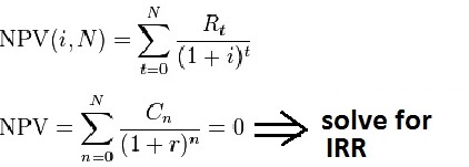
Return, Risk
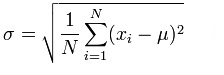
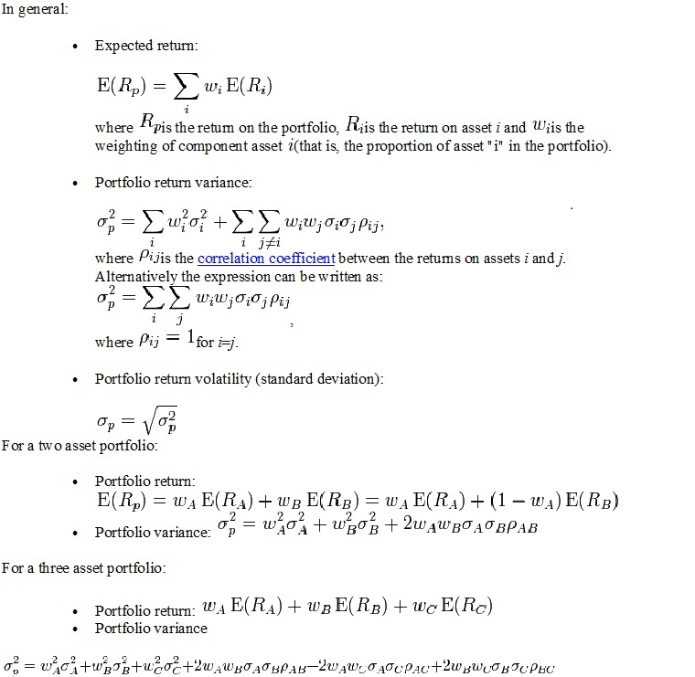
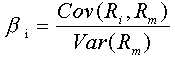
Dividend Growth Model
Po= D1/(r-g) or Po= Do*(1+g)/(r-g)
R
= D1/Po+g = Do*(1+g)/Po+g
D1=Do*(1+g);
D2= D1*(1+g)…
WACC
WACC = weight of debt * cost of debt + weight
of equity *( cost of equity)
Wd= total debt / Total capital = total borrowed /
total capital
We= total equity/ Total capital
Cost of debt = rate(nper, coupon, -(price – flotation costs),
1000)*(1-tax rate)
Cost of Equity = D1/(Po – Flotation Cost) +
g
D1: Next period dividend; Po: Current stock price; g: dividend
growth rate
Note: flotation costs = flotation percentage * price
Or if beta is given, use CAPM model (refer to chapter 6)
Cost of equity = risk free rate + beta *(market return – risk
free rate)
Cost of equity = risk free rate + beta * market risk premium